- The Space Environment

Содержание
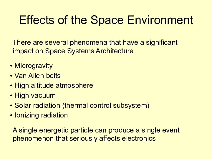
- 2. Effects of the Space Environment There are several phenomena that have a significant impact on Space
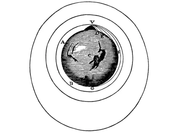
- 4. The gravitational field Obviously, all satellites in orbit around the Earth (or any other object) are
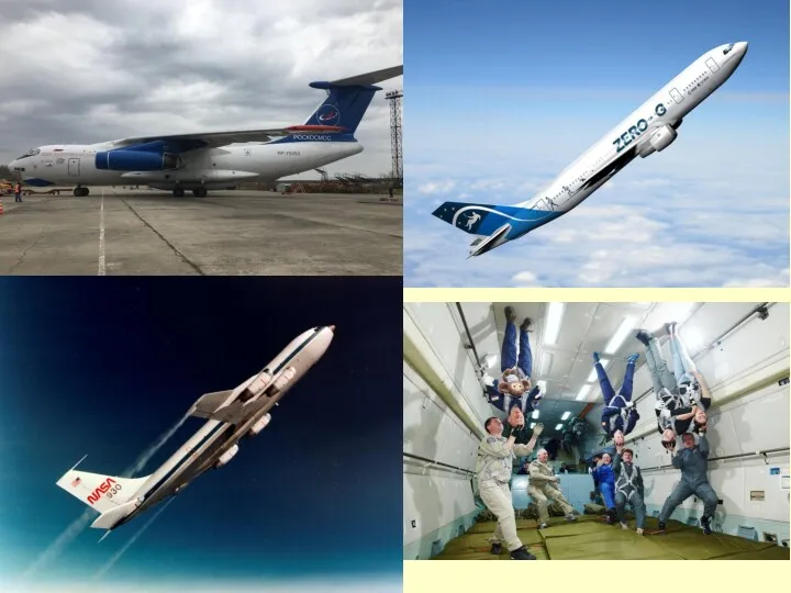
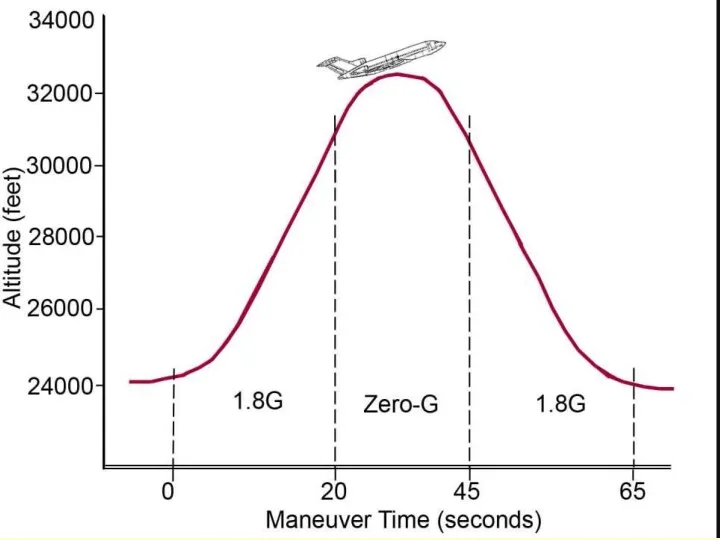
- 6. Simulating microgravity Then, it is possible to simulate microgravity by letting fall an object (better in
- 8. Interior of the Bremen test tower
- 11. ESA’s REXUS rocket
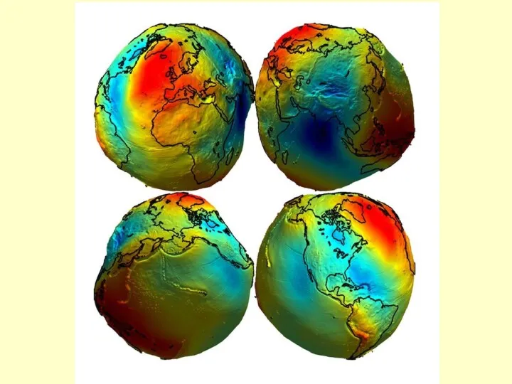
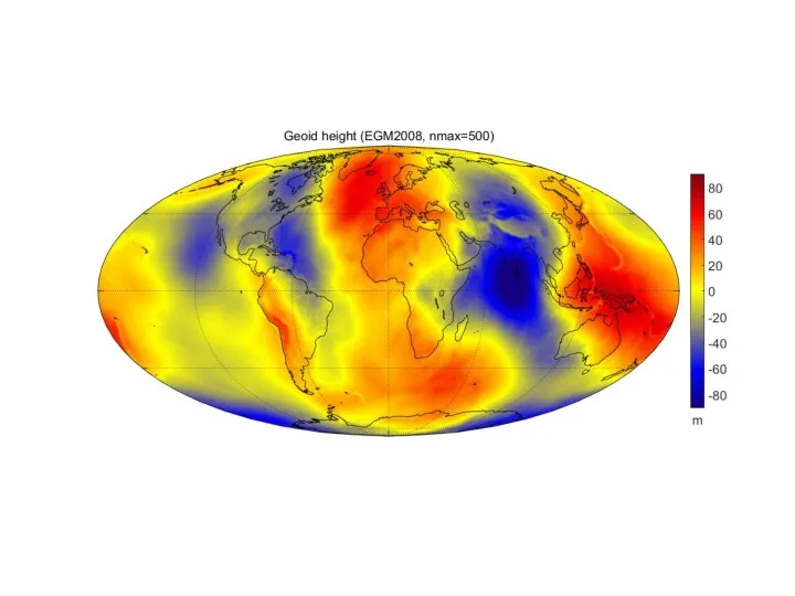
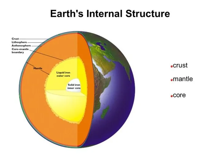
- 13. Gravitational field
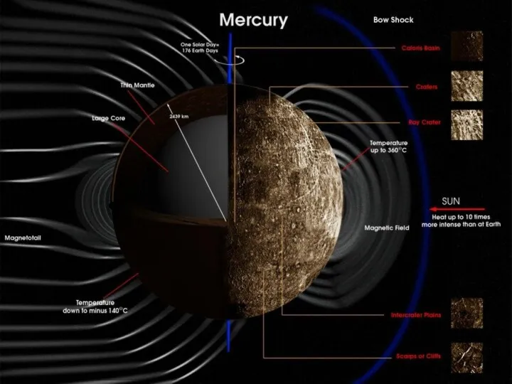
- 16. Other celestial bodies have, obviously, different gravitational fields
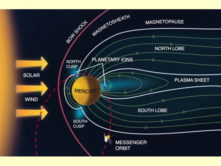
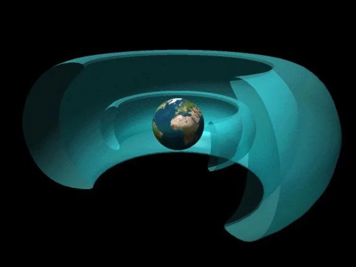
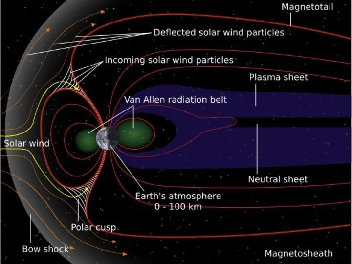
- 17. The magnetosphere and radiation belts The Earth is surrounded by radiation belts of energetic particles trapped
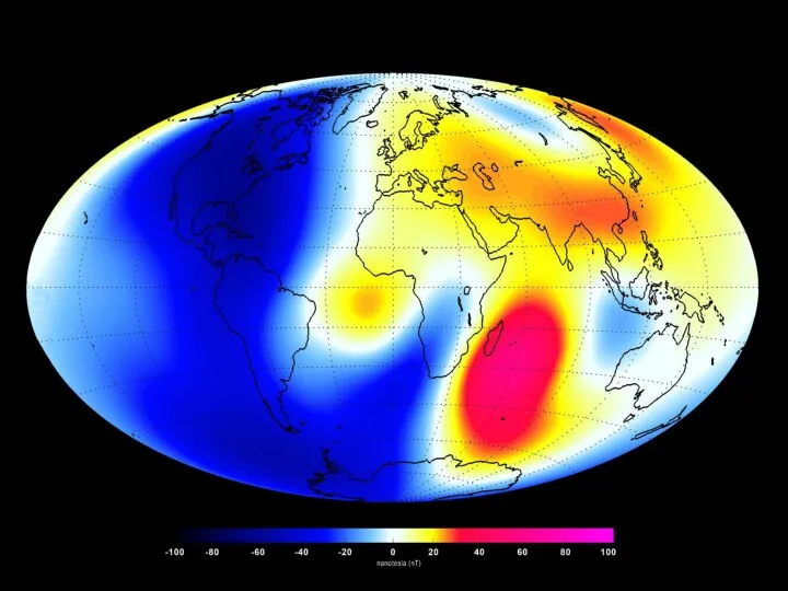
- 20. IGRF12
- 28. Geometry and physical explanation of trapped radiation belts
- 31. Models for radiation belts Proton models: Solar minimum: AP8MIN Solar Maximum: AP8MAX Electron models Solar minimum:
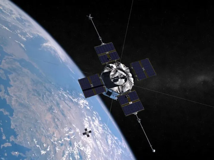
- 32. The third van Allen belt Recently, the van Allen probes have discovered a third (transient) van
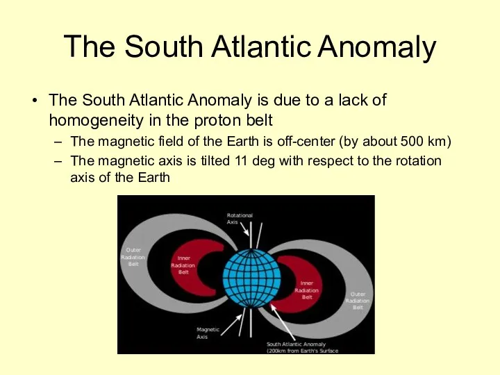
- 35. The South Atlantic Anomaly The South Atlantic Anomaly is due to a lack of homogeneity in
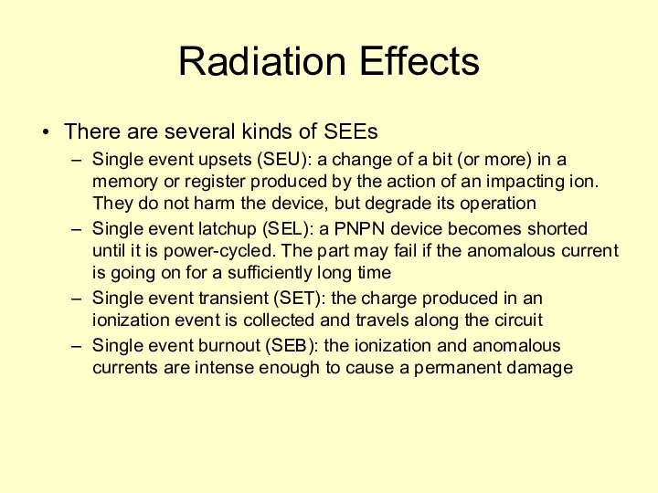
- 36. Radiation Effects There are several kinds of SEEs Single event upsets (SEU): a change of a
- 37. Images of the South Atlantic Anomaly
- 38. The effects of SAA The South Atlantic Anomaly is due to a lack of homogeneity in
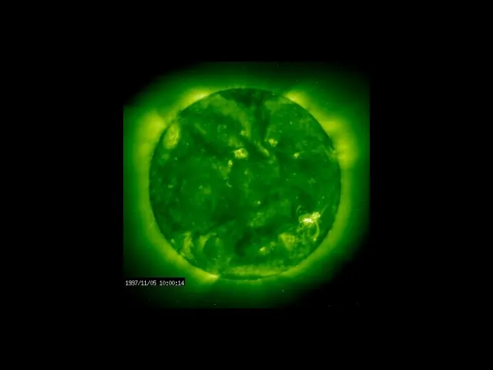
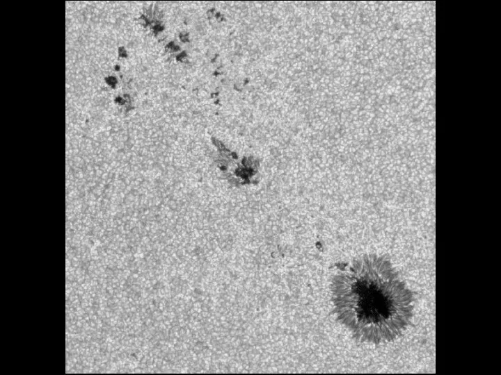
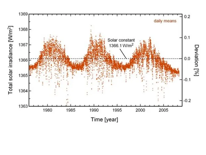
- 40. The Solar Cycle The Sun experiences substantial changes in its activity with a period of ~11.2
- 43. Variation of the F10.7 index throughout the last 60 years
- 44. The structure of the F10.7 peaks is highly variable and difficult to predict
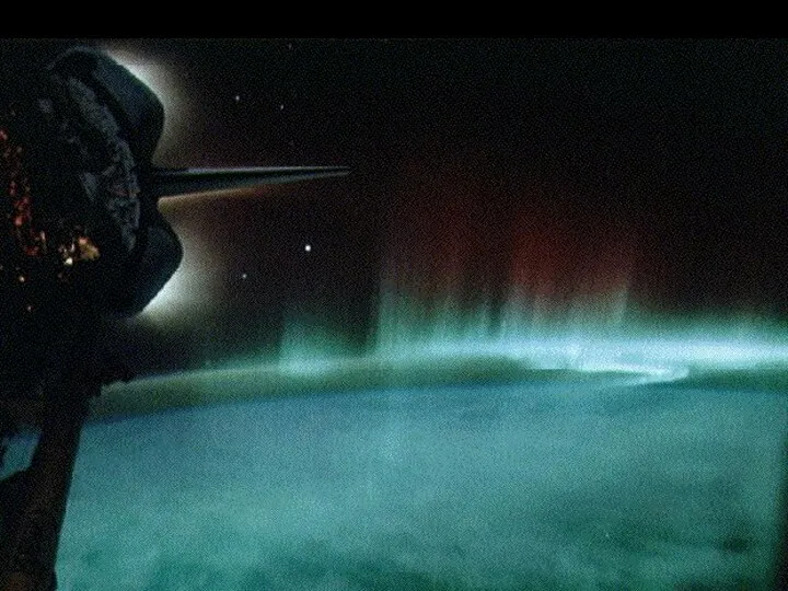
- 47. The Upper Atmosphere The atmosphere has no clear limits in height (but legally ends at 100
- 48. The Upper Atmosphere For most satellites CD ≈ 1.90 – 2.60 The presence of solar panels
- 49. Maxwell-Boltzmann Distribution
- 50. Maxwell-Boltzmann Distribution
- 52. Knudsen number Measures whether the satellite moves in a continuum medium (Kn 10) It is defined
- 57. The Upper Atmosphere The Upper atmosphere is affected by the intensity of solar and geomagnetic activity
- 58. Effects of the Upper Atmosphere Aerodynamic drag which can lead to orbit decay Depends of ballistic
- 60. Mass = 7 kg Apogee = 2581 km Diameter = 3.7 m Perigee = 635 km
- 61. Effects of the Upper Atmosphere Aerodynamic drag which can lead to orbit decay Depends of ballistic
- 62. A Swarm of Femtosatellites to Determine the Density of the Lower Thermosphere Carlos Lledó Jordi L.
- 63. Why study the thermosphere? The thermosphere extends from 90 to approximately 600 km The region of
- 64. Similar missions POPACS (Polar Orbiting Passive Atmospheric Calibration Spheres) Three 0.1 m spheres of 1.0, 1.5,
- 65. Direct density determination
- 66. noon midnight F10.7= 50,100,200 m=0.1 kg, CD=2.2 d=5 cm BC = 5.8 kg/m2 NRL-MSISE00 model
- 67. Our project Our plan is to set up a swarm of tens to hundreds of spherical
- 68. The femtosatellite (1)
- 69. The femtosatellite (2) Omnidirectional antenna Only Tx mode No ADCS subsystem Passive thermal control + aerogel
- 70. Electronics layout of the femtosatellite
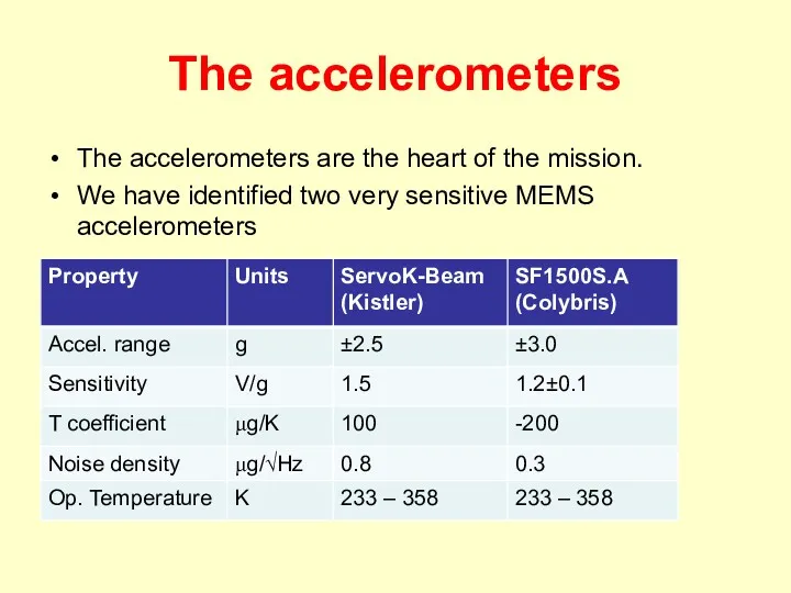
- 71. The accelerometers The accelerometers are the heart of the mission. We have identified two very sensitive
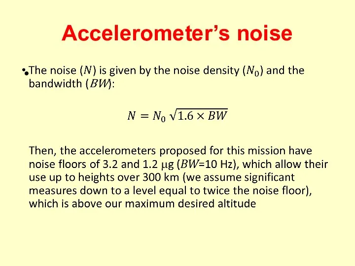
- 72. Accelerometer’s noise
- 73. Noon midnight F10.7= 50,100,200 Continuous line: noise floor dot-dashed line: twice noise floor m=0.1 kg, CD=2.2
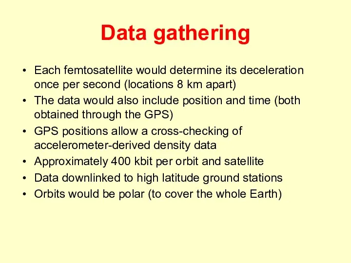
- 74. Data gathering Each femtosatellite would determine its deceleration once per second (locations 8 km apart) The
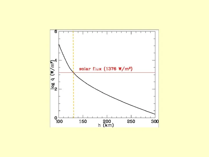
- 75. Thermal control
- 77. Noise sources and uncertainties Rotational state of the satellites Non-orthogonality of the 1D accelerometers (cross-linking) Drag
- 78. Open problems Launch and dispersion of a truly Earth-covering swarm Accelerometer testing Battery’s limited endurance (“Remove
- 79. Conclusions and future work The mission seams feasible Launch and dispersion still an issue Accelerometer testing
- 80. Mass and power budgets
- 81. M=0.1 kg, CD=2.2 D=5 cm
- 82. The swarm as a space debris hazard A large swarm could be seen as a potential
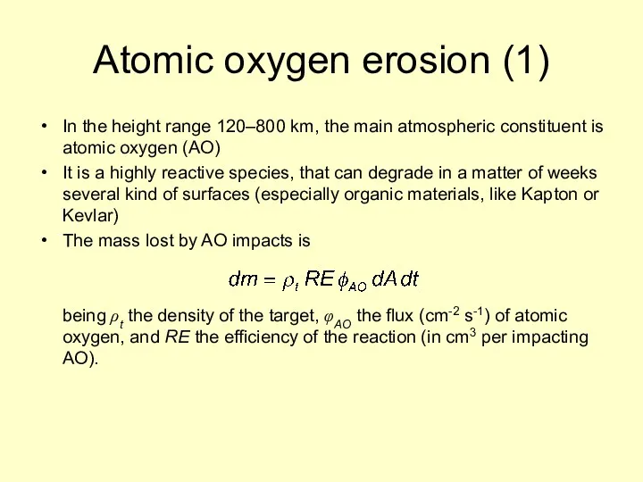
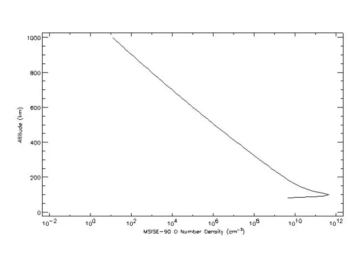
- 83. Atomic oxygen erosion (1) In the height range 120–800 km, the main atmospheric constituent is atomic
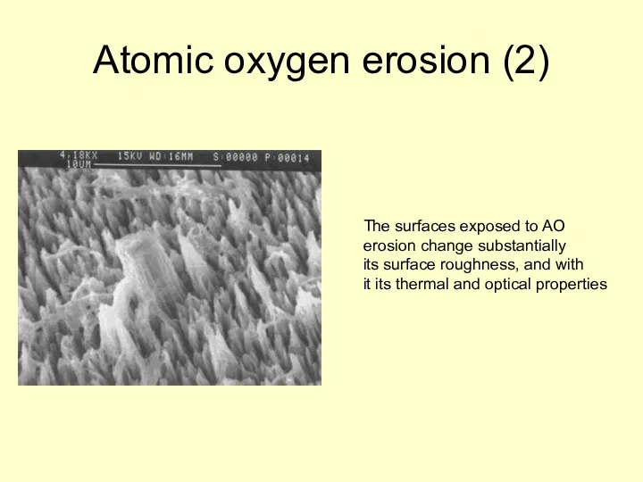
- 85. Atomic oxygen erosion (2) The surfaces exposed to AO erosion change substantially its surface roughness, and
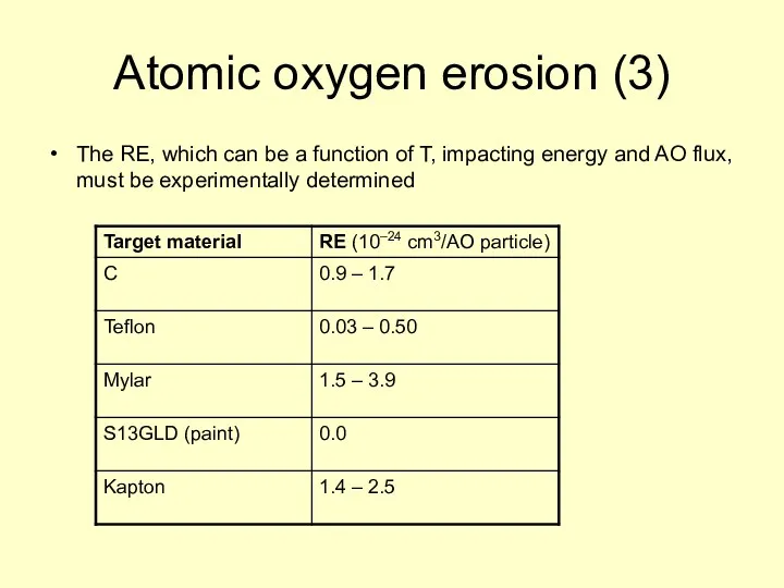
- 86. Atomic oxygen erosion (3) The RE, which can be a function of T, impacting energy and
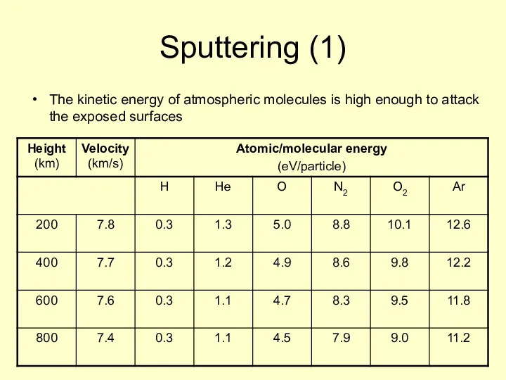
- 87. Sputtering (1) The kinetic energy of atmospheric molecules is high enough to attack the exposed surfaces
- 88. Sputtering (2) Sputtering (in the case of an intense ion beam) Effects of sputtering on the
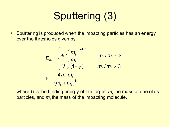
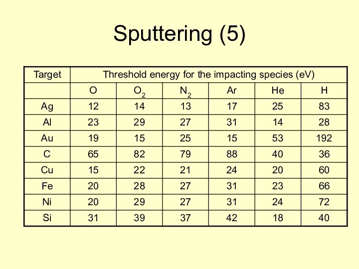
- 89. Sputtering (3) Sputtering is produced when the impacting particles has an energy over the thresholds given
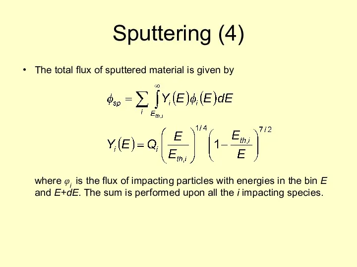
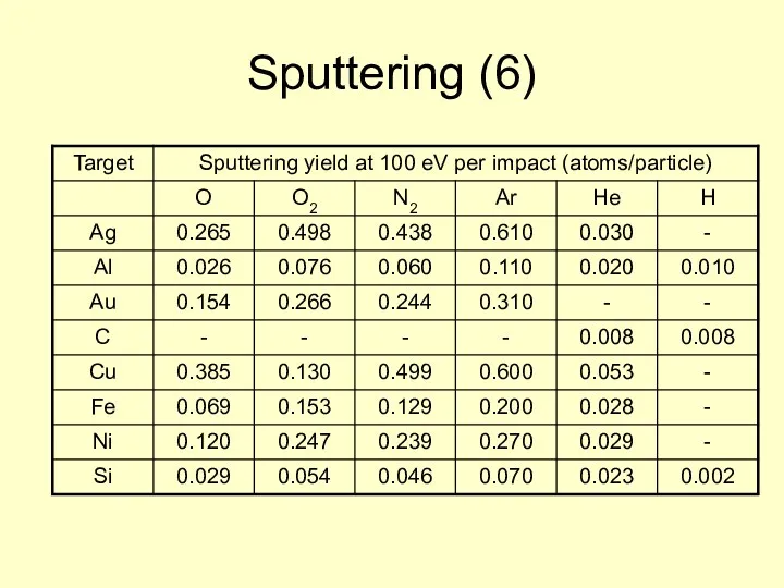
- 90. Sputtering (4) The total flux of sputtered material is given by where φi is the flux
- 91. Sputtering (5)
- 92. Sputtering (6)
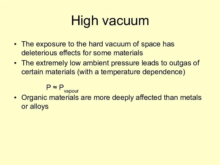
- 93. High vacuum The exposure to the hard vacuum of space has deleterious effects for some materials
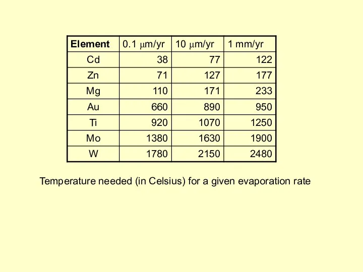
- 94. Temperature needed (in Celsius) for a given evaporation rate
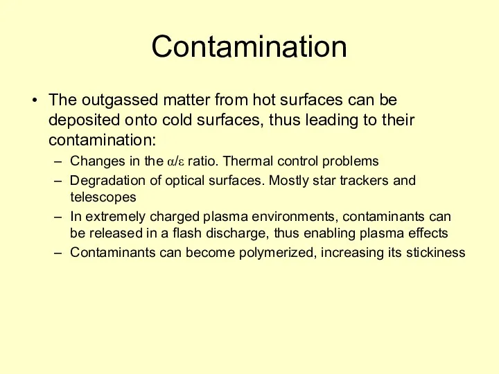
- 95. Contamination The outgassed matter from hot surfaces can be deposited onto cold surfaces, thus leading to
- 96. The effects of vacuum exposure At 100 km in height the pressure is ~0.1 Pa, and
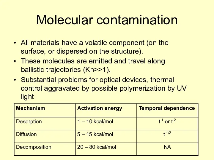
- 97. Molecular contamination All materials have a volatile component (on the surface, or dispersed on the structure).
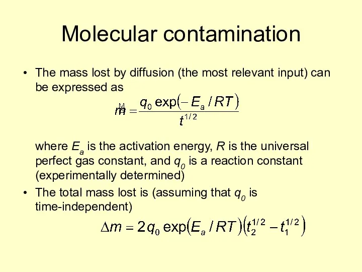
- 98. Molecular contamination The mass lost by diffusion (the most relevant input) can be expressed as where
- 99. Molecular contamination transport The amount of mass transferred to a specific point of the satellite from
- 100. Molecular contamination deposition A molecule impacting a surface can get stuck for a characteristic time given
- 101. ASTM E595 This is a test to determine the Total Mass Loss (TML), the Collected Volatile
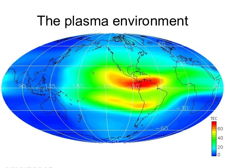
- 102. The plasma environment At heights over ~100 km the radiation of the Sun ionizes the main
- 103. The plasma environment
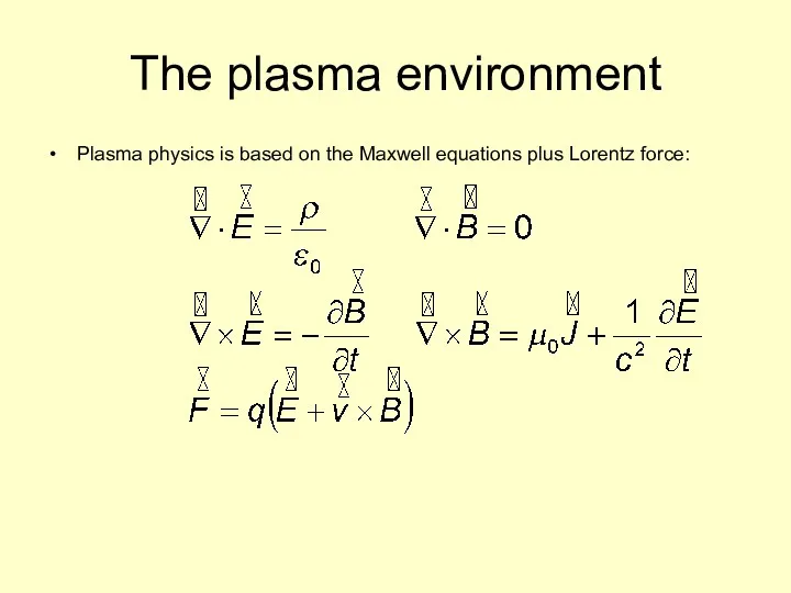
- 104. The plasma environment Plasma physics is based on the Maxwell equations plus Lorentz force:
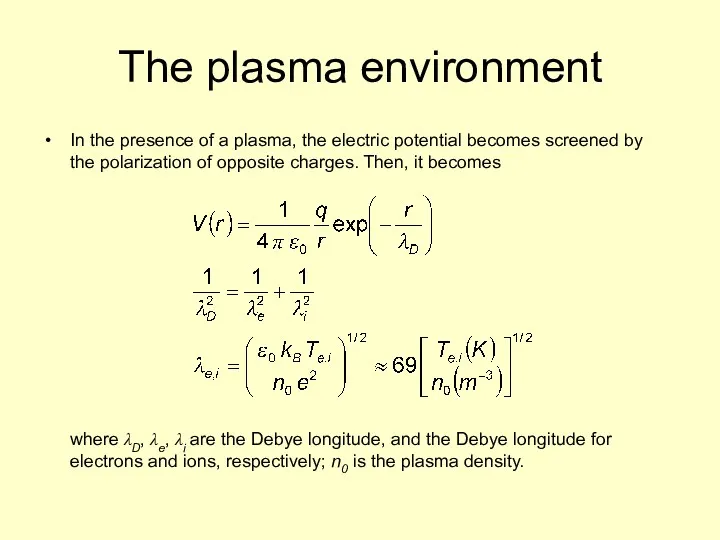
- 105. The plasma environment In the presence of a plasma, the electric potential becomes screened by the
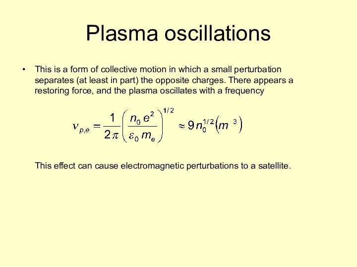
- 106. Plasma oscillations This is a form of collective motion in which a small perturbation separates (at
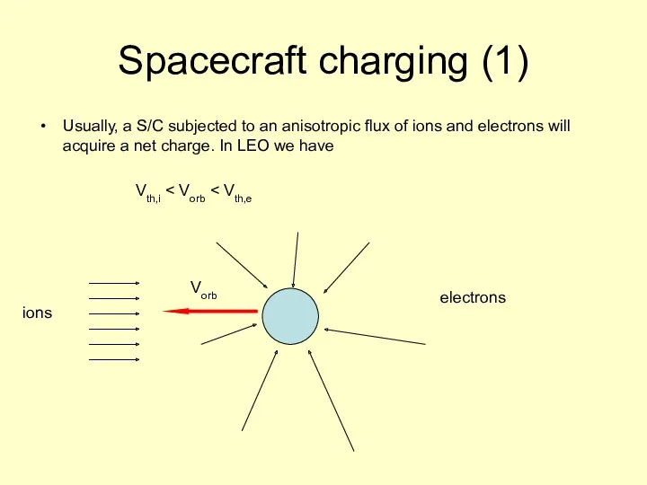
- 107. Spacecraft charging (1) Usually, a S/C subjected to an anisotropic flux of ions and electrons will
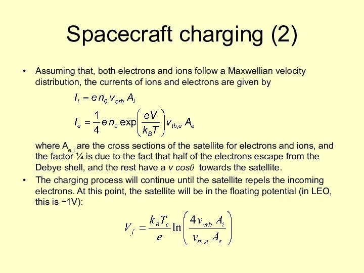
- 108. Spacecraft charging (2) Assuming that, both electrons and ions follow a Maxwellian velocity distribution, the currents
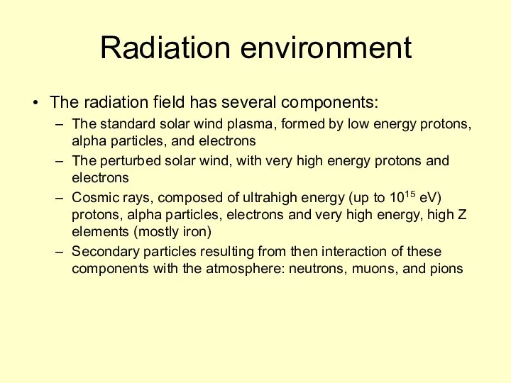
- 109. Radiation environment The radiation field has several components: The standard solar wind plasma, formed by low
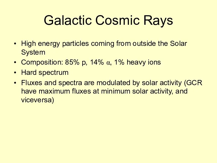
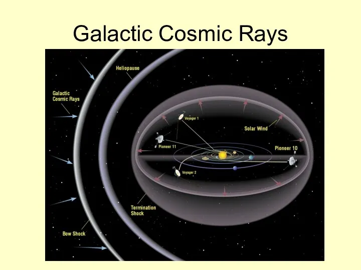
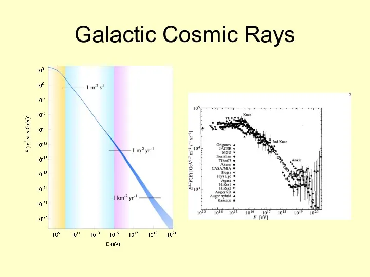
- 110. Galactic Cosmic Rays High energy particles coming from outside the Solar System Composition: 85% p, 14%
- 111. Galactic Cosmic Rays
- 112. Galactic Cosmic Rays
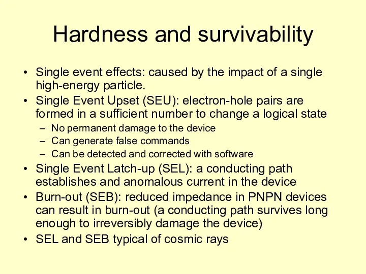
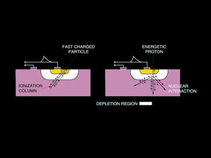
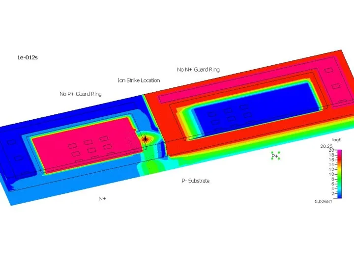
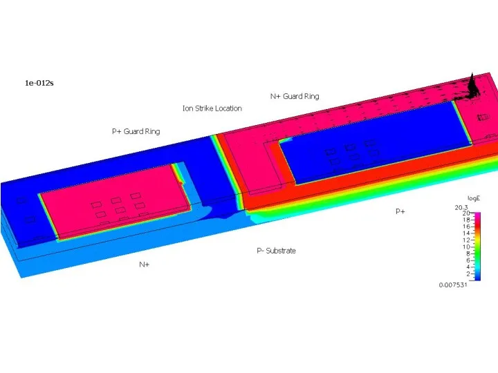
- 113. Hardness and survivability Single event effects: caused by the impact of a single high-energy particle. Single
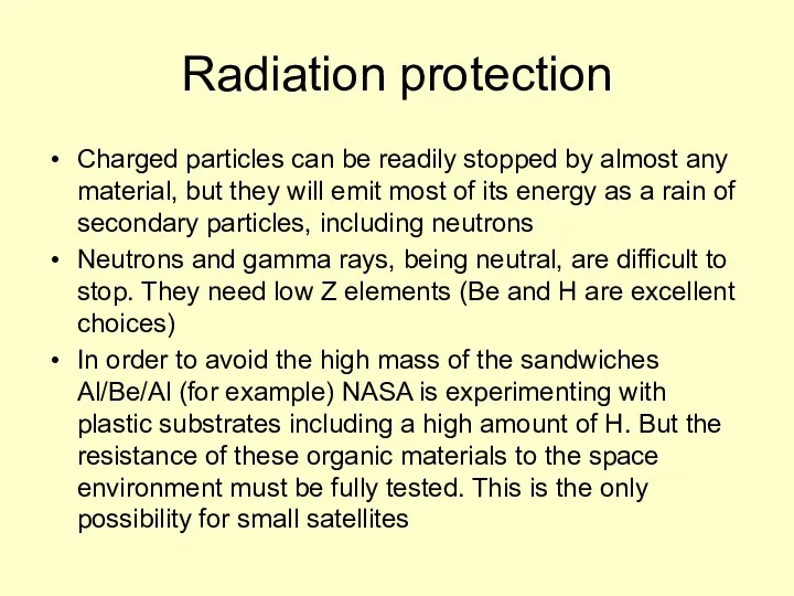
- 117. Radiation protection Charged particles can be readily stopped by almost any material, but they will emit
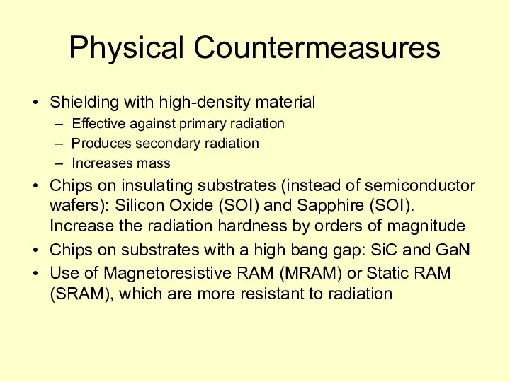
- 118. Physical Countermeasures Shielding with high-density material Effective against primary radiation Produces secondary radiation Increases mass Chips
- 119. Software Countermeasures Error-Correcting Code (ECC): Uses parity bits to identify alterations Continuous reading of memory to
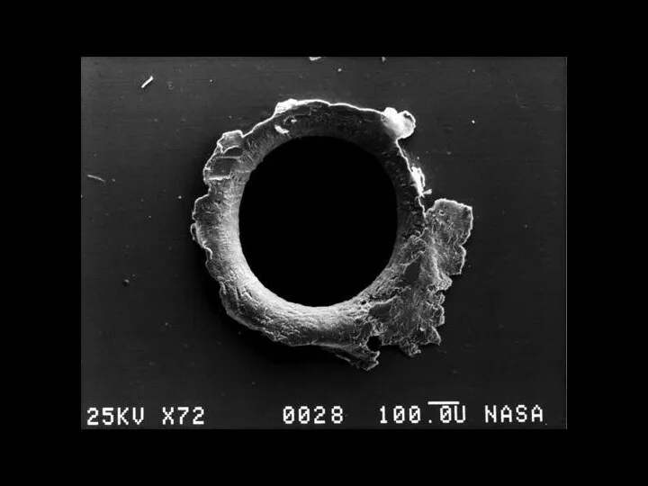
- 120. Micrometeoroids (1) Micrometeoroids (and space debris) do not usually destroy a satellite, but in the long
- 121. Micrometeoroids (2) The flux of micrometeoroids is given by where m is the mass of the
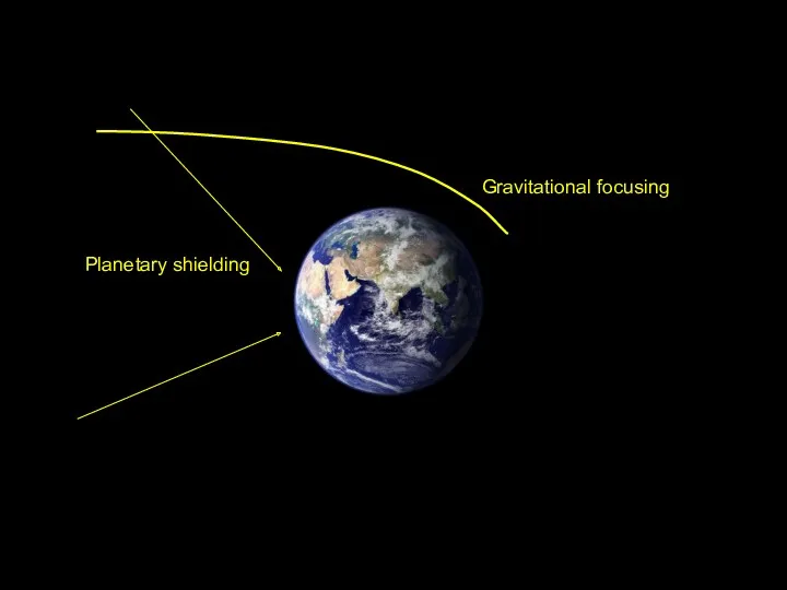
- 122. Micrometeoroids (3) And also acts as a shield Most impacts are produced on the space-facing surfaces
- 123. Gravitational focusing Planetary shielding
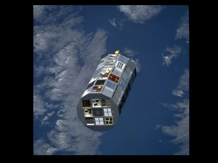
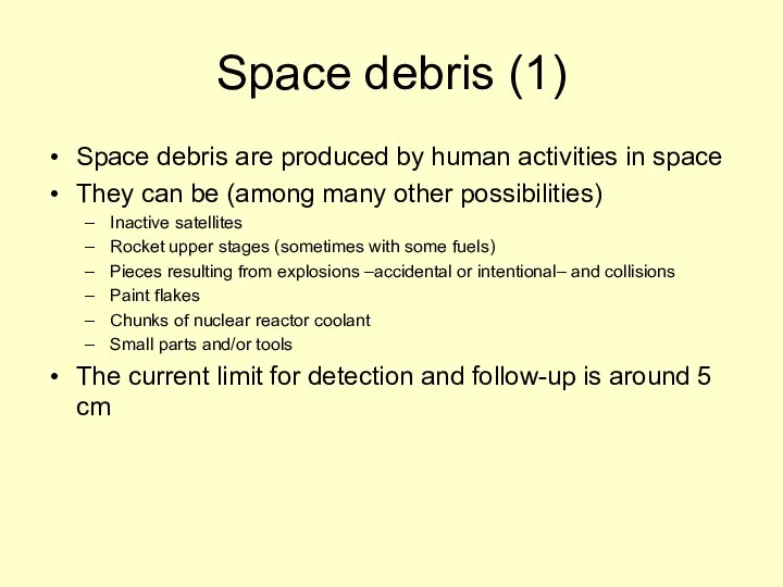
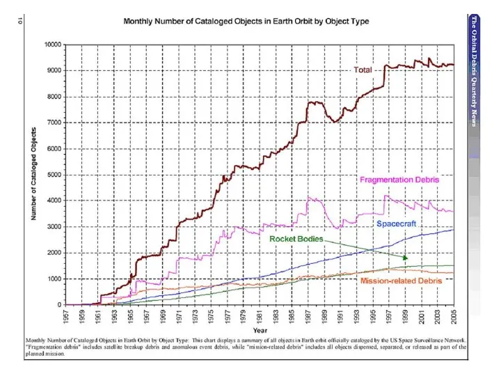
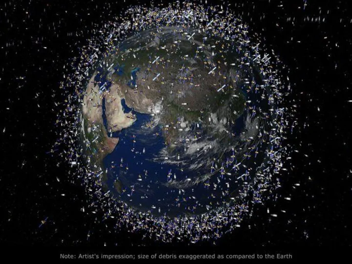
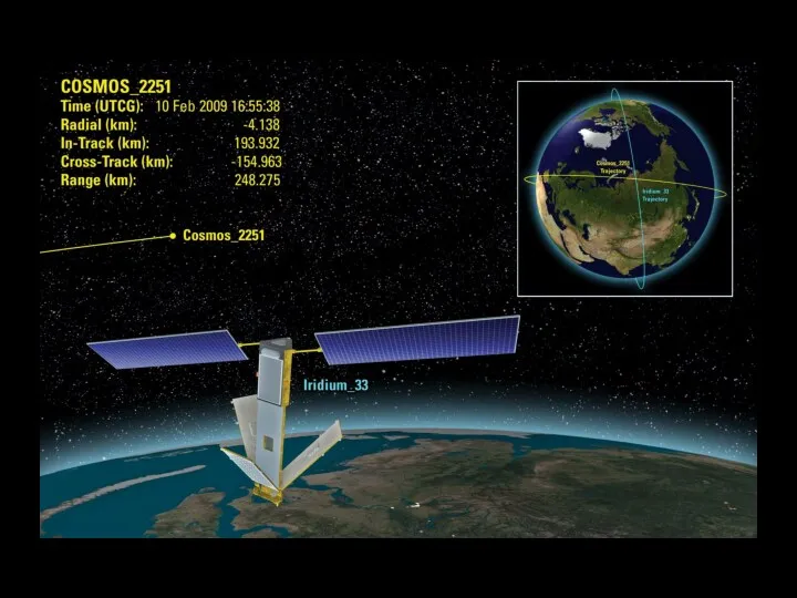
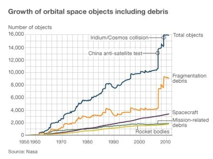
- 126. Space debris (1) Space debris are produced by human activities in space They can be (among
- 133. Space debris (2) Space debris at heights of less than 600 km reenter in the atmosphere
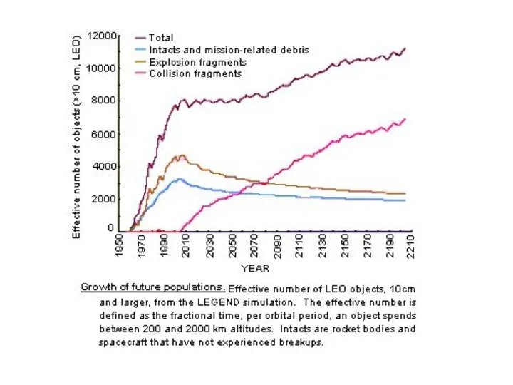
- 134. Kessler syndrome It is possible that a series of collisions between space debris produces a cascade
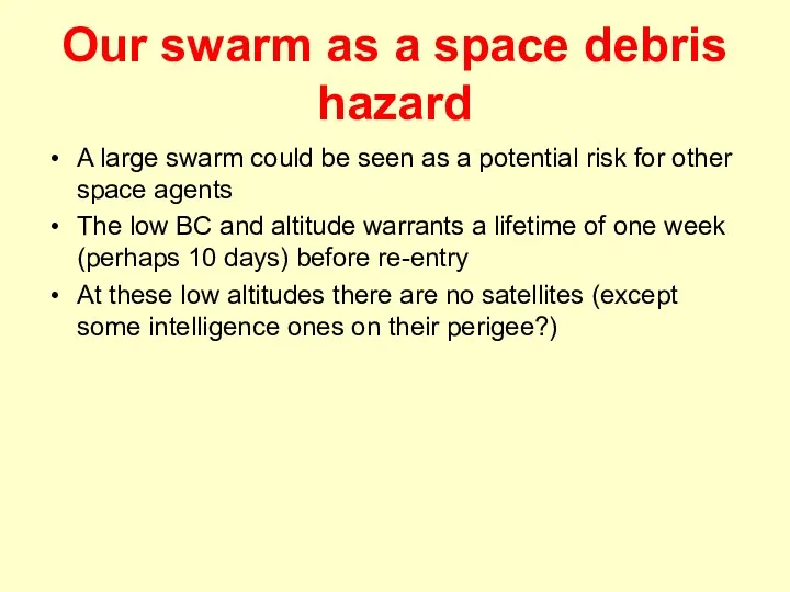
- 135. Our swarm as a space debris hazard A large swarm could be seen as a potential
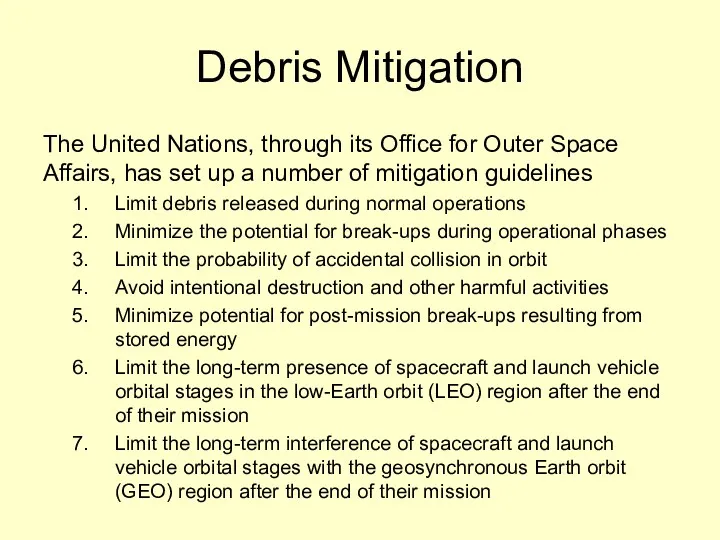
- 137. Debris Mitigation The United Nations, through its Office for Outer Space Affairs, has set up a
- 138. References General references Alan C. Tribble, The Space Environment, Princeton University Press (2003) Vincent L. Pisacane,
- 139. References Atomic Oxygen Erosion Zhan, Y., & Zhang, G., Low Earth orbit environmental effects on materials,
- 141. Скачать презентацию
Effects of the Space Environment
There are several phenomena that have a
Effects of the Space Environment
There are several phenomena that have a
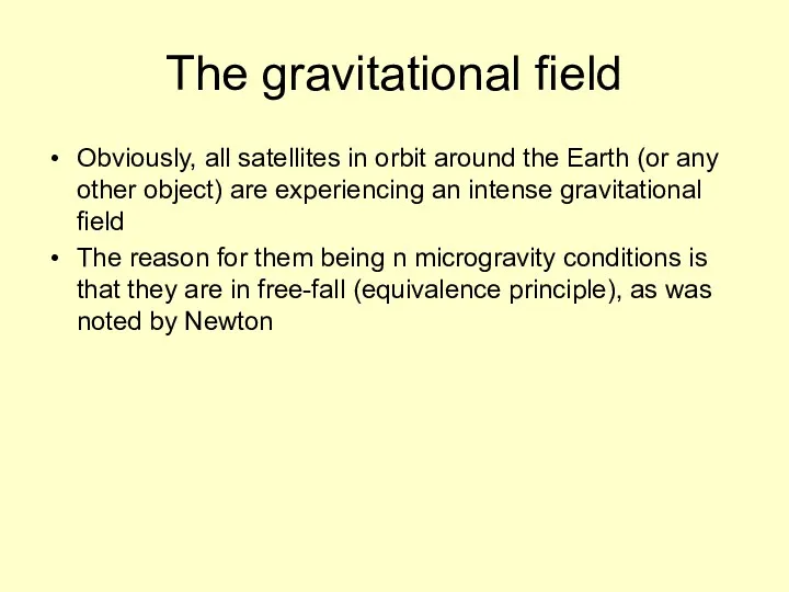
The gravitational field
Obviously, all satellites in orbit around the Earth (or
The gravitational field
Obviously, all satellites in orbit around the Earth (or
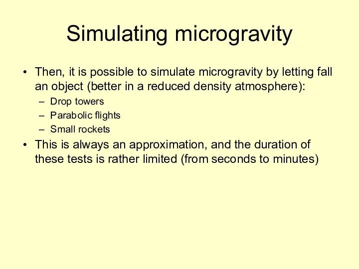
Simulating microgravity
Then, it is possible to simulate microgravity by letting fall
Simulating microgravity
Then, it is possible to simulate microgravity by letting fall
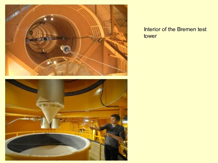
Interior of the Bremen test
tower
Interior of the Bremen test
tower
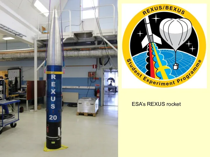
ESA’s REXUS rocket
ESA’s REXUS rocket
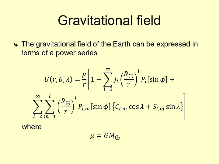
Gravitational field
Gravitational field
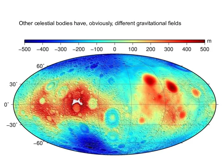
Other celestial bodies have, obviously, different gravitational fields
Other celestial bodies have, obviously, different gravitational fields
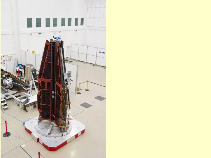
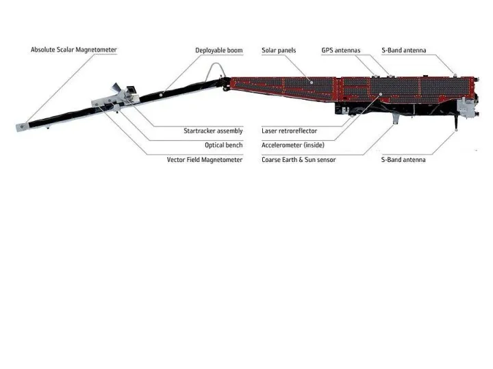
The magnetosphere and
radiation belts
The Earth is surrounded by radiation belts
The magnetosphere and
radiation belts
The Earth is surrounded by radiation belts
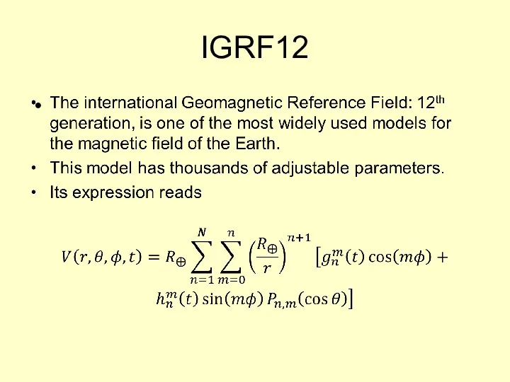
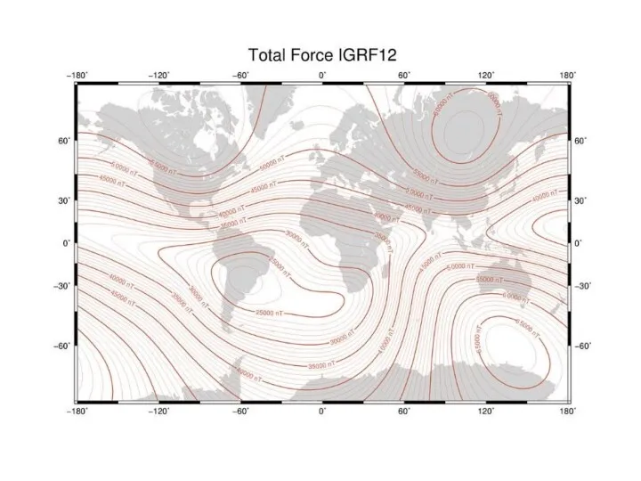
IGRF12
IGRF12
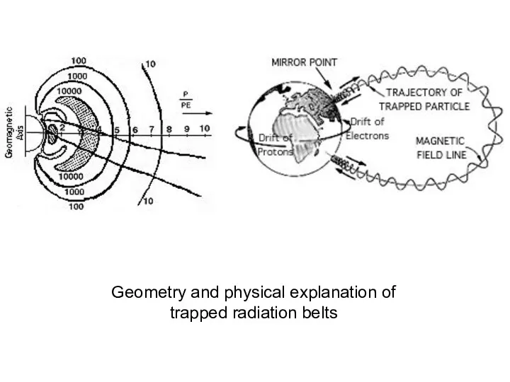
Geometry and physical explanation of
trapped radiation belts
Geometry and physical explanation of
trapped radiation belts
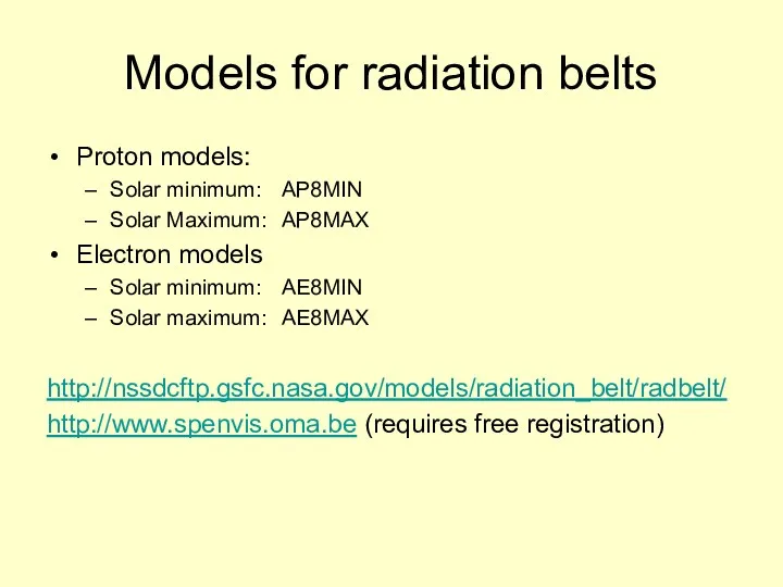
Models for radiation belts
Proton models:
Solar minimum: AP8MIN
Solar Maximum: AP8MAX
Electron models
Solar minimum: AE8MIN
Solar
Models for radiation belts
Proton models:
Solar minimum: AP8MIN
Solar Maximum: AP8MAX
Electron models
Solar minimum: AE8MIN
Solar
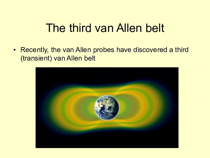
The third van Allen belt
Recently, the van Allen probes have discovered
The third van Allen belt
Recently, the van Allen probes have discovered
The South Atlantic Anomaly
The South Atlantic Anomaly is due to a
The South Atlantic Anomaly
The South Atlantic Anomaly is due to a
Radiation Effects
There are several kinds of SEEs
Single event upsets (SEU): a
Radiation Effects
There are several kinds of SEEs
Single event upsets (SEU): a
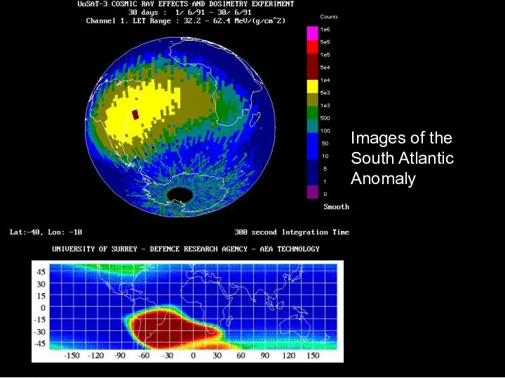
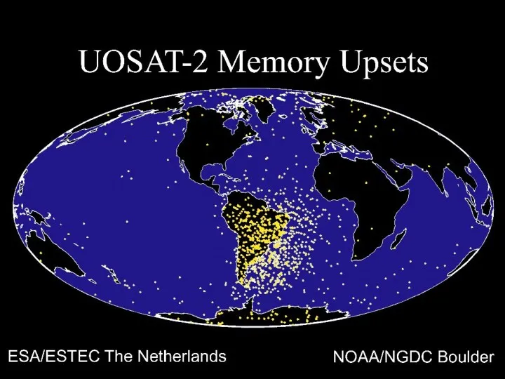
Images of the South Atlantic Anomaly
Images of the South Atlantic Anomaly
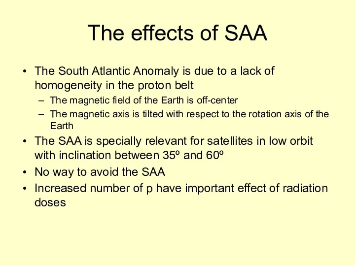
The effects of SAA
The South Atlantic Anomaly is due to a
The effects of SAA
The South Atlantic Anomaly is due to a
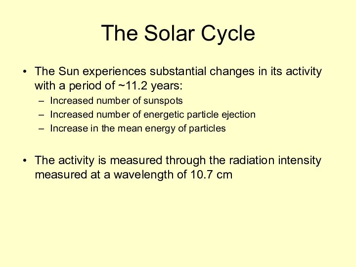
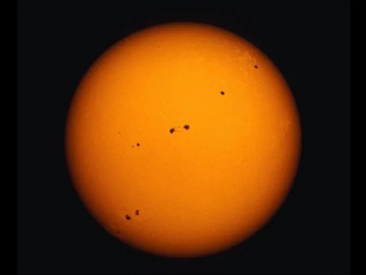
The Solar Cycle
The Sun experiences substantial changes in its activity with
The Solar Cycle
The Sun experiences substantial changes in its activity with
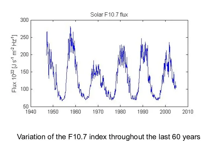
Variation of the F10.7 index throughout the last 60 years
Variation of the F10.7 index throughout the last 60 years
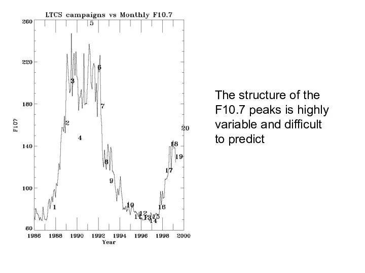
The structure of the
F10.7 peaks is highly
variable and difficult
to predict
The structure of the
F10.7 peaks is highly
variable and difficult
to predict
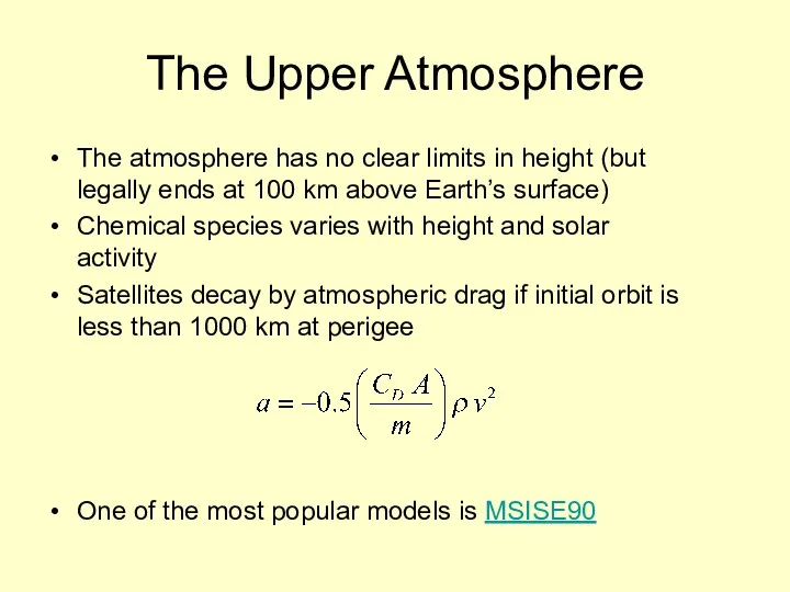
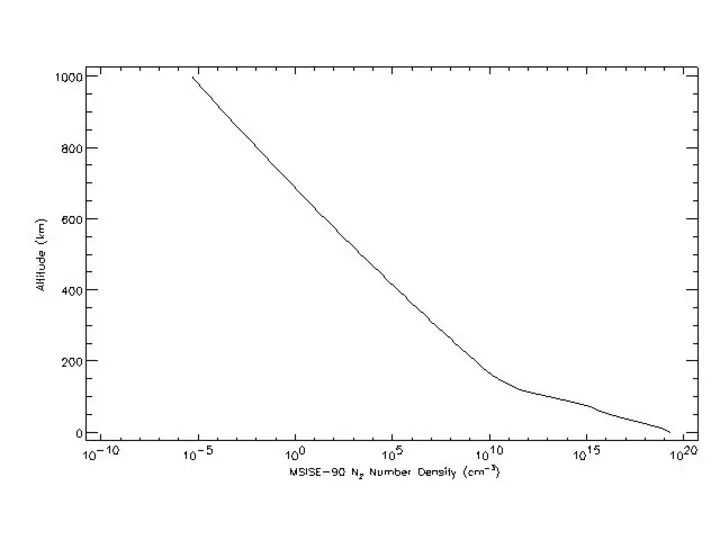
The Upper Atmosphere
The atmosphere has no clear limits in height (but
The Upper Atmosphere
The atmosphere has no clear limits in height (but
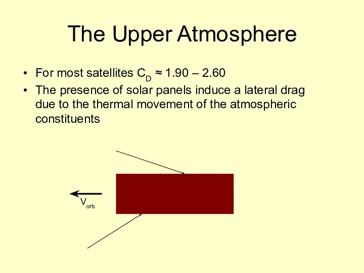
The Upper Atmosphere
For most satellites CD ≈ 1.90 – 2.60
The presence
The Upper Atmosphere
For most satellites CD ≈ 1.90 – 2.60
The presence
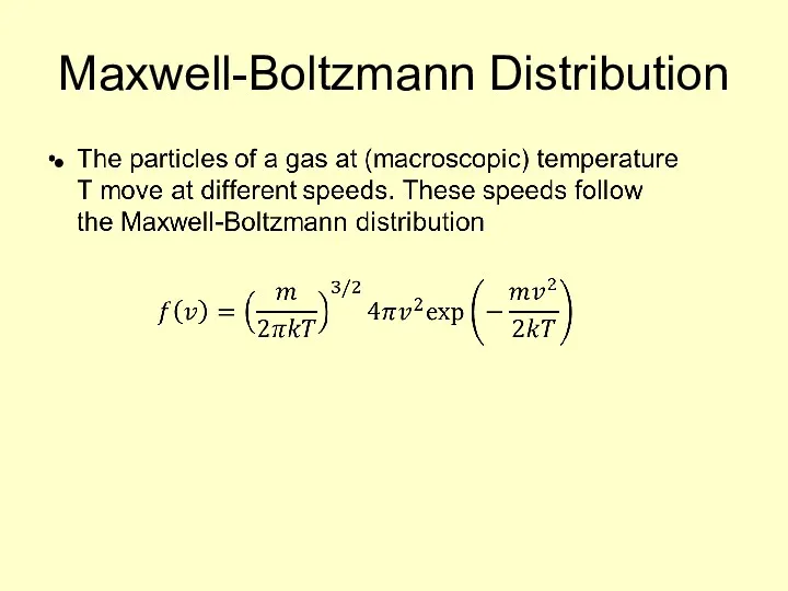
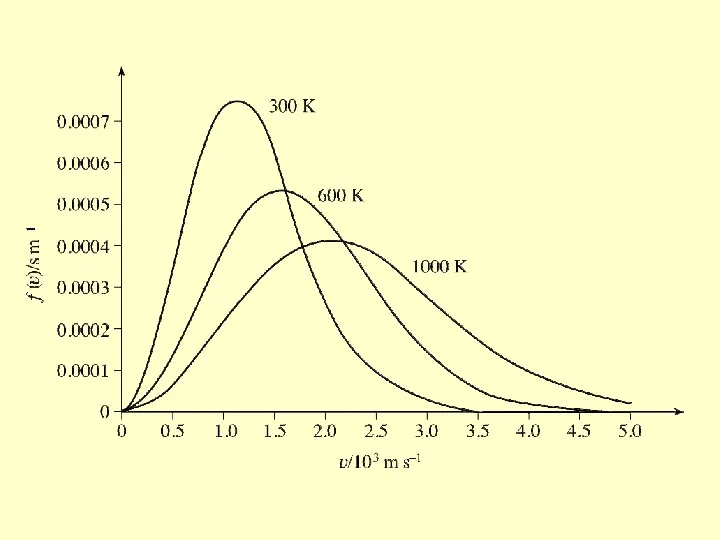
Maxwell-Boltzmann Distribution
Maxwell-Boltzmann Distribution
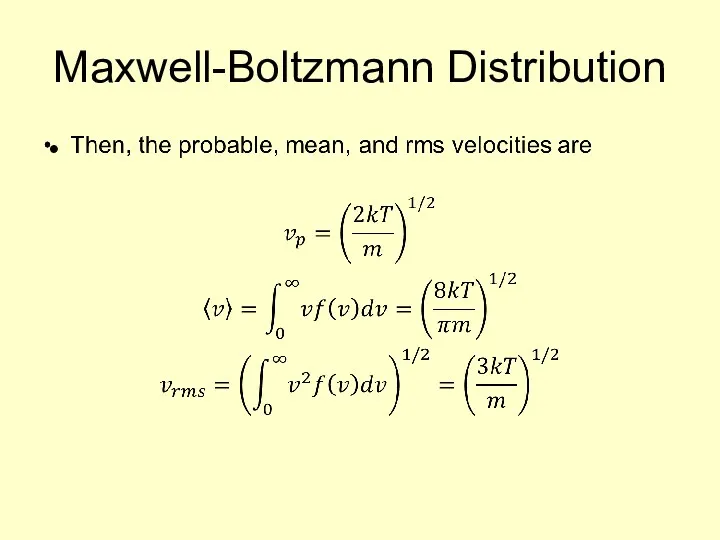
Maxwell-Boltzmann Distribution
Maxwell-Boltzmann Distribution
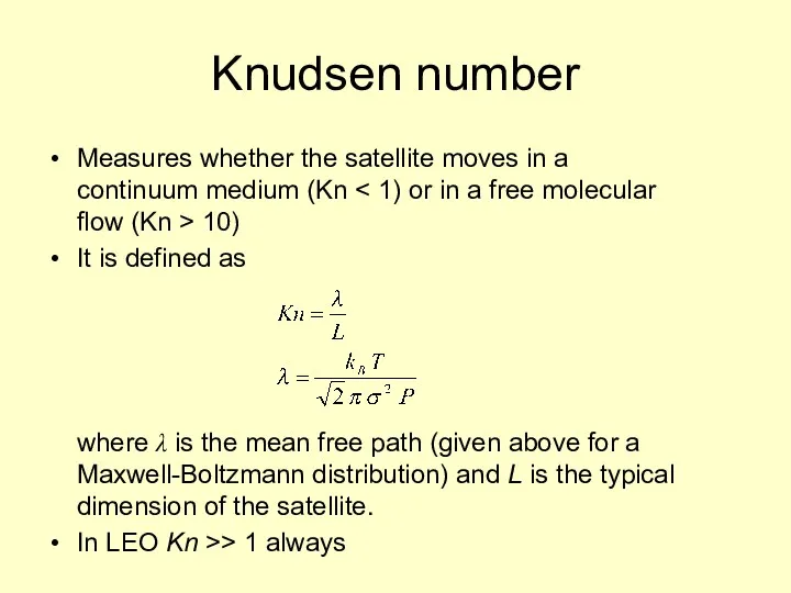
Knudsen number
Measures whether the satellite moves in a continuum medium (Kn
Knudsen number
Measures whether the satellite moves in a continuum medium (Kn

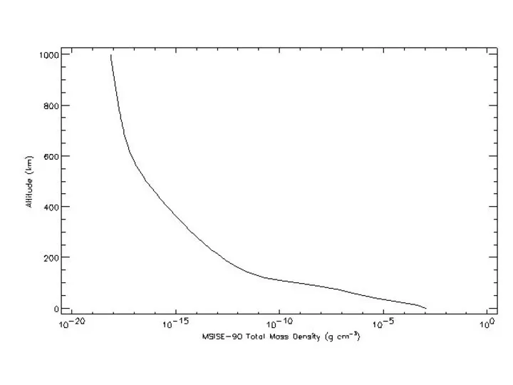
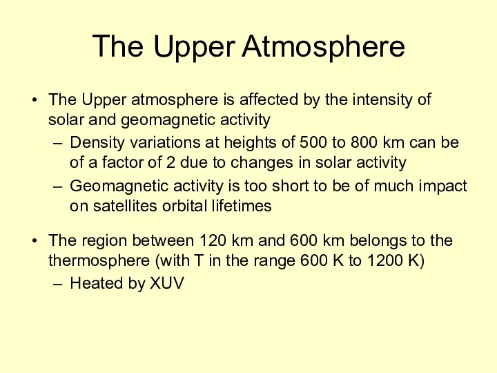
The Upper Atmosphere
The Upper atmosphere is affected by the intensity of
The Upper Atmosphere
The Upper atmosphere is affected by the intensity of
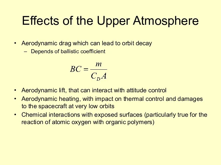
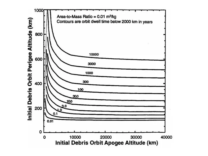
Effects of the Upper Atmosphere
Aerodynamic drag which can lead to orbit
Effects of the Upper Atmosphere
Aerodynamic drag which can lead to orbit
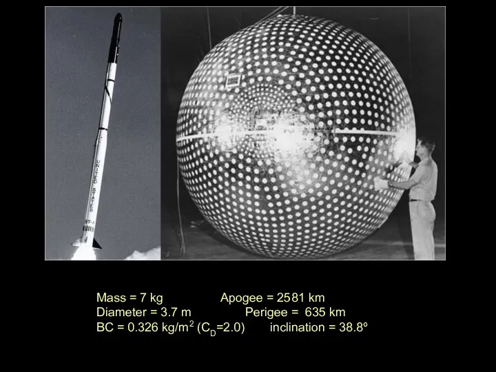
Mass = 7 kg Apogee = 2581 km
Diameter = 3.7 m Perigee =
Mass = 7 kg Apogee = 2581 km
Diameter = 3.7 m Perigee =
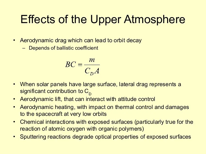
Effects of the Upper Atmosphere
Aerodynamic drag which can lead to orbit
Effects of the Upper Atmosphere
Aerodynamic drag which can lead to orbit
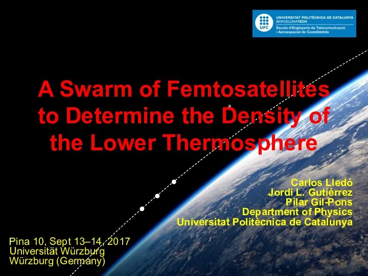
A Swarm of Femtosatellites to Determine the Density of the Lower
A Swarm of Femtosatellites to Determine the Density of the Lower
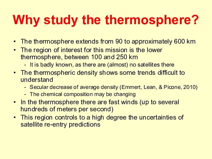
Why study the thermosphere?
The thermosphere extends from 90 to approximately 600
Why study the thermosphere?
The thermosphere extends from 90 to approximately 600
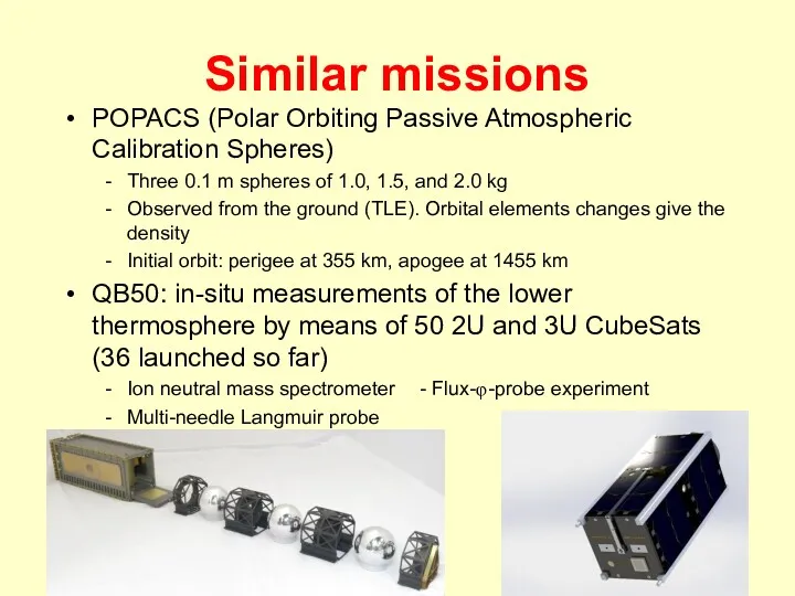
Similar missions
POPACS (Polar Orbiting Passive Atmospheric Calibration Spheres)
Three 0.1 m spheres
Similar missions
POPACS (Polar Orbiting Passive Atmospheric Calibration Spheres)
Three 0.1 m spheres
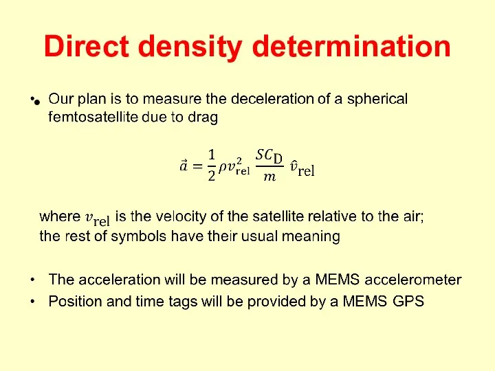
Direct density determination
Direct density determination
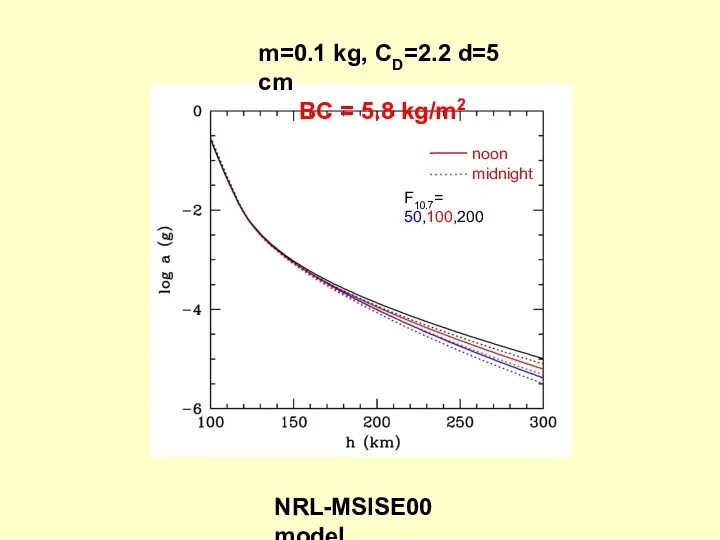
noon
midnight
F10.7= 50,100,200
m=0.1 kg, CD=2.2 d=5 cm
BC = 5.8 kg/m2
NRL-MSISE00 model
noon
midnight
F10.7= 50,100,200
m=0.1 kg, CD=2.2 d=5 cm
BC = 5.8 kg/m2
NRL-MSISE00 model
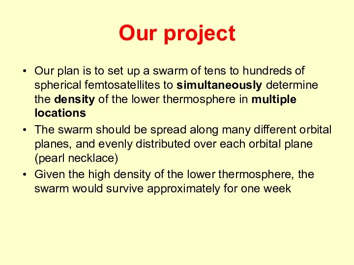
Our project
Our plan is to set up a swarm of tens
Our project
Our plan is to set up a swarm of tens
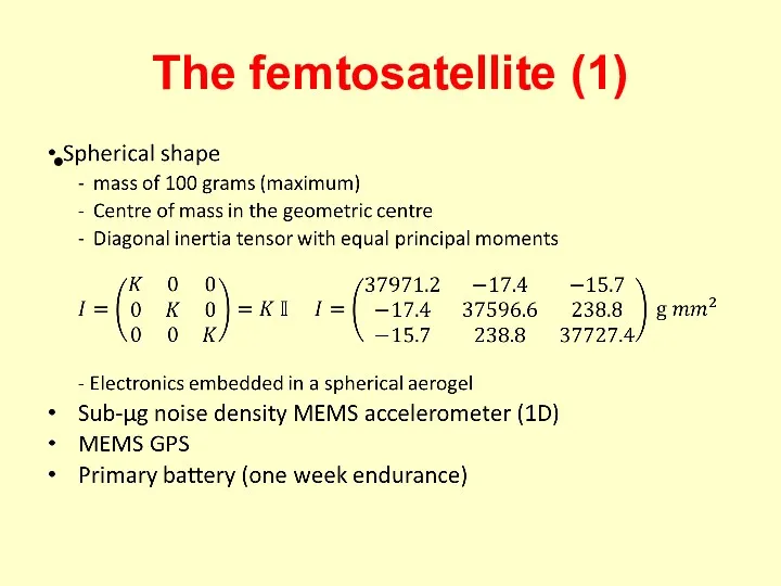
The femtosatellite (1)
The femtosatellite (1)
The femtosatellite (2)
Omnidirectional antenna
Only Tx mode
No ADCS subsystem
Passive thermal control +
The femtosatellite (2)
Omnidirectional antenna
Only Tx mode
No ADCS subsystem
Passive thermal control +
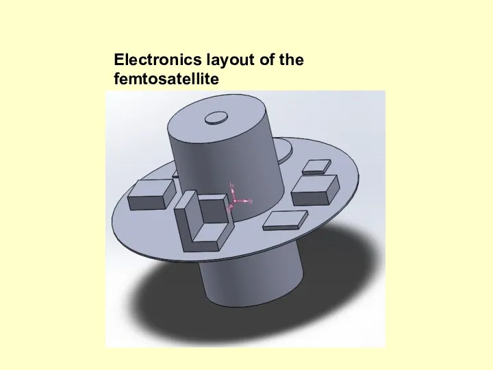
Electronics layout of the femtosatellite
Electronics layout of the femtosatellite
The accelerometers
The accelerometers are the heart of the mission.
We have identified
The accelerometers
The accelerometers are the heart of the mission.
We have identified
Accelerometer’s noise
Accelerometer’s noise
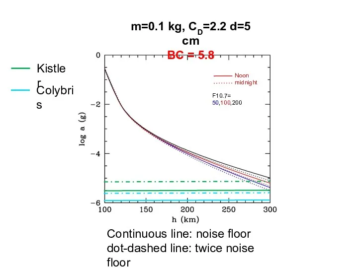
Noon
midnight
F10.7= 50,100,200
Continuous line: noise floor
dot-dashed line: twice noise floor
m=0.1 kg, CD=2.2
Noon
midnight
F10.7= 50,100,200
Continuous line: noise floor
dot-dashed line: twice noise floor
m=0.1 kg, CD=2.2
Data gathering
Each femtosatellite would determine its deceleration once per second (locations
Data gathering
Each femtosatellite would determine its deceleration once per second (locations
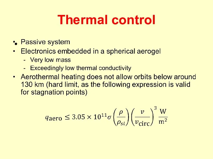
Thermal control
Thermal control
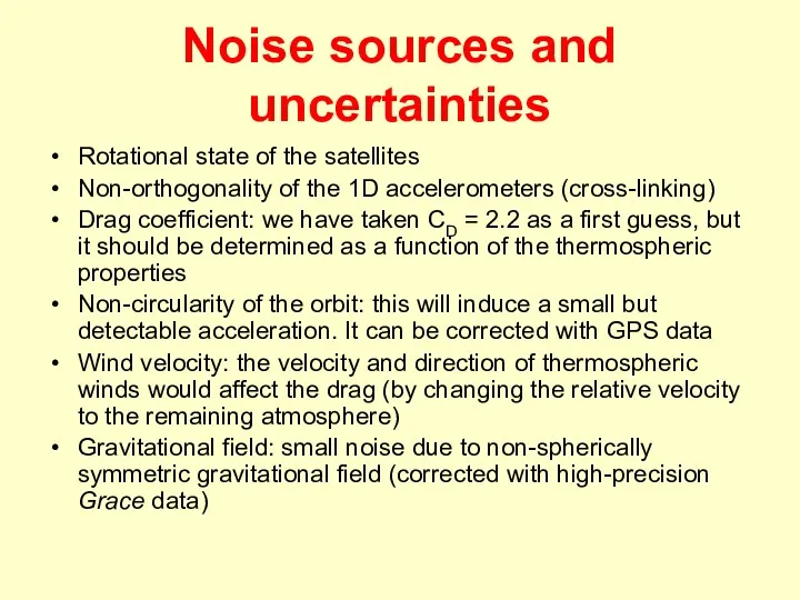
Noise sources and uncertainties
Rotational state of the satellites
Non-orthogonality of the 1D
Noise sources and uncertainties
Rotational state of the satellites
Non-orthogonality of the 1D
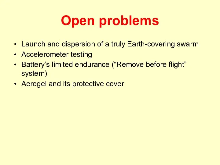
Open problems
Launch and dispersion of a truly Earth-covering swarm
Accelerometer testing
Battery’s limited
Open problems
Launch and dispersion of a truly Earth-covering swarm
Accelerometer testing
Battery’s limited
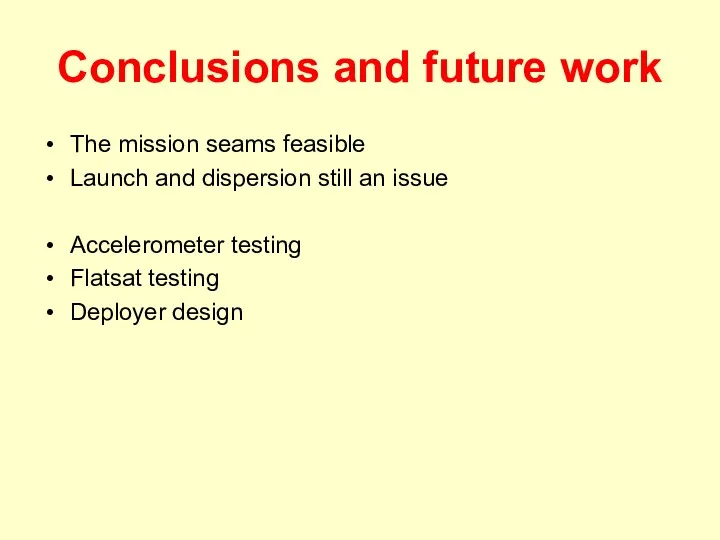
Conclusions and future work
The mission seams feasible
Launch and dispersion still an
Conclusions and future work
The mission seams feasible
Launch and dispersion still an
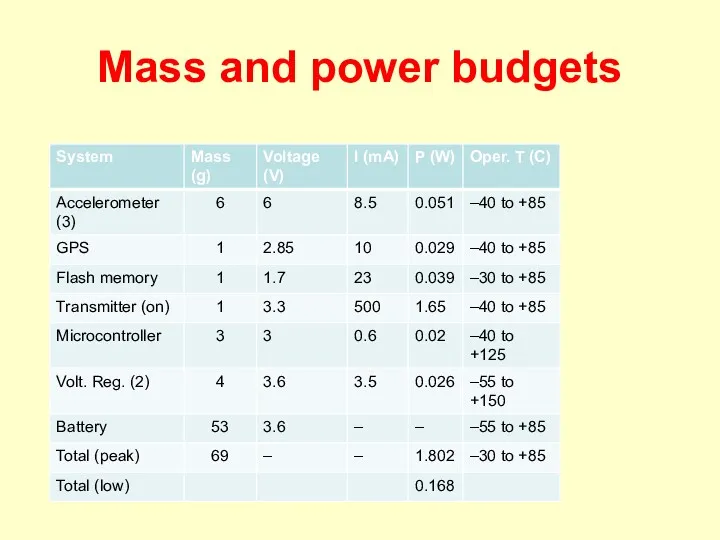
Mass and power budgets
Mass and power budgets
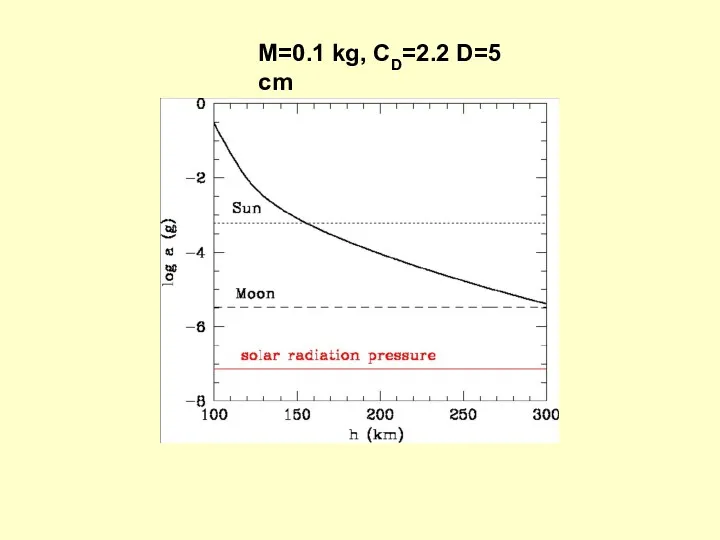
M=0.1 kg, CD=2.2 D=5 cm
M=0.1 kg, CD=2.2 D=5 cm
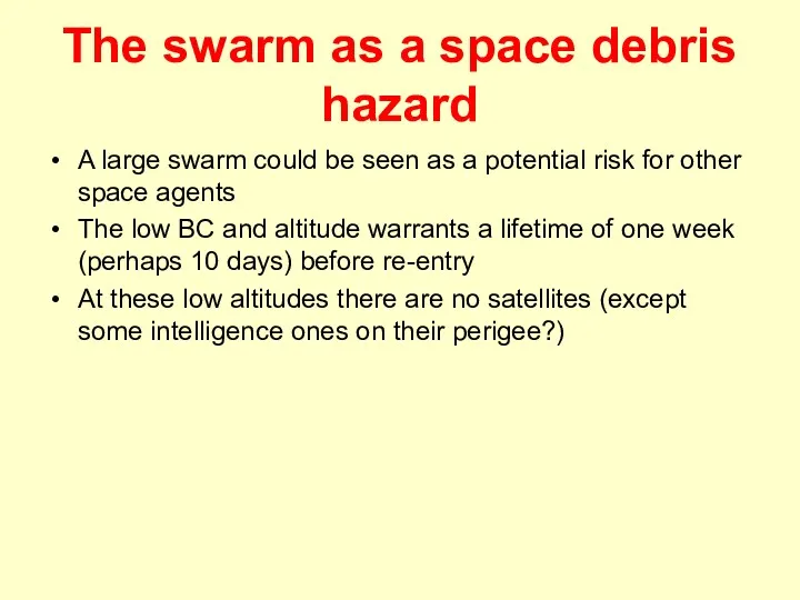
The swarm as a space debris hazard
A large swarm could be
The swarm as a space debris hazard
A large swarm could be
Atomic oxygen erosion (1)
In the height range 120–800 km, the main
Atomic oxygen erosion (1)
In the height range 120–800 km, the main
Atomic oxygen erosion (2)
The surfaces exposed to AO
erosion change substantially
its
Atomic oxygen erosion (2)
The surfaces exposed to AO
erosion change substantially
its
Atomic oxygen erosion (3)
The RE, which can be a function of
Atomic oxygen erosion (3)
The RE, which can be a function of
Sputtering (1)
The kinetic energy of atmospheric molecules is high enough to
Sputtering (1)
The kinetic energy of atmospheric molecules is high enough to
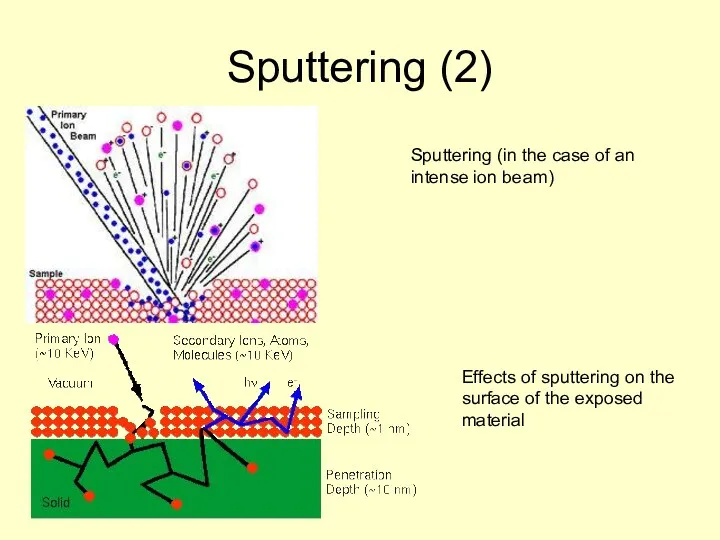
Sputtering (2)
Sputtering (in the case of an
intense ion beam)
Effects of sputtering
Sputtering (2)
Sputtering (in the case of an
intense ion beam)
Effects of sputtering
Sputtering (3)
Sputtering is produced when the impacting particles has an energy
Sputtering (3)
Sputtering is produced when the impacting particles has an energy
Sputtering (4)
The total flux of sputtered material is given by
where φi
Sputtering (4)
The total flux of sputtered material is given by
where φi
Sputtering (5)
Sputtering (5)
Sputtering (6)
Sputtering (6)
High vacuum
The exposure to the hard vacuum of space has deleterious
High vacuum
The exposure to the hard vacuum of space has deleterious
Temperature needed (in Celsius) for a given evaporation rate
Temperature needed (in Celsius) for a given evaporation rate
Contamination
The outgassed matter from hot surfaces can be deposited onto cold
Contamination
The outgassed matter from hot surfaces can be deposited onto cold
The effects of vacuum exposure
At 100 km in height the pressure
The effects of vacuum exposure
At 100 km in height the pressure
Molecular contamination
All materials have a volatile component (on the surface, or
Molecular contamination
All materials have a volatile component (on the surface, or
Molecular contamination
The mass lost by diffusion (the most relevant input) can
Molecular contamination
The mass lost by diffusion (the most relevant input) can
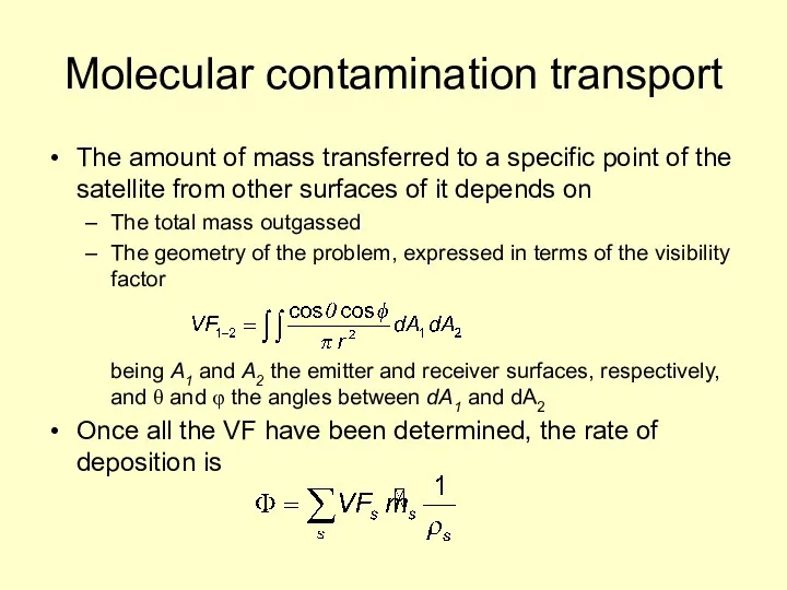
Molecular contamination transport
The amount of mass transferred to a specific point
Molecular contamination transport
The amount of mass transferred to a specific point
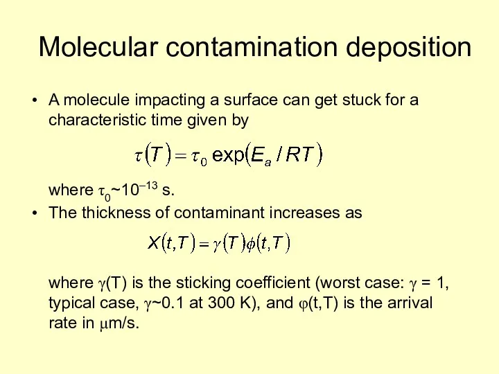
Molecular contamination deposition
A molecule impacting a surface can get stuck for
Molecular contamination deposition
A molecule impacting a surface can get stuck for
ASTM E595
This is a test to determine the Total Mass Loss
ASTM E595
This is a test to determine the Total Mass Loss
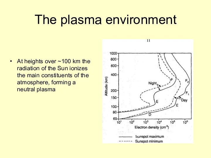
The plasma environment
At heights over ~100 km the radiation of the
The plasma environment
At heights over ~100 km the radiation of the
The plasma environment
The plasma environment
The plasma environment
Plasma physics is based on the Maxwell equations plus
The plasma environment
Plasma physics is based on the Maxwell equations plus
The plasma environment
In the presence of a plasma, the electric potential
The plasma environment
In the presence of a plasma, the electric potential
Plasma oscillations
This is a form of collective motion in which a
Plasma oscillations
This is a form of collective motion in which a
Spacecraft charging (1)
Usually, a S/C subjected to an anisotropic flux of
Spacecraft charging (1)
Usually, a S/C subjected to an anisotropic flux of
Spacecraft charging (2)
Assuming that, both electrons and ions follow a Maxwellian
Spacecraft charging (2)
Assuming that, both electrons and ions follow a Maxwellian
Radiation environment
The radiation field has several components:
The standard solar wind plasma,
Radiation environment
The radiation field has several components:
The standard solar wind plasma,
Galactic Cosmic Rays
High energy particles coming from outside the Solar System
Composition:
Galactic Cosmic Rays
High energy particles coming from outside the Solar System
Composition:
Galactic Cosmic Rays
Galactic Cosmic Rays
Galactic Cosmic Rays
Galactic Cosmic Rays
Hardness and survivability
Single event effects: caused by the impact of a
Hardness and survivability
Single event effects: caused by the impact of a
Radiation protection
Charged particles can be readily stopped by almost any material,
Radiation protection
Charged particles can be readily stopped by almost any material,
Physical Countermeasures
Shielding with high-density material
Effective against primary radiation
Produces secondary radiation
Increases mass
Chips
Physical Countermeasures
Shielding with high-density material
Effective against primary radiation
Produces secondary radiation
Increases mass
Chips
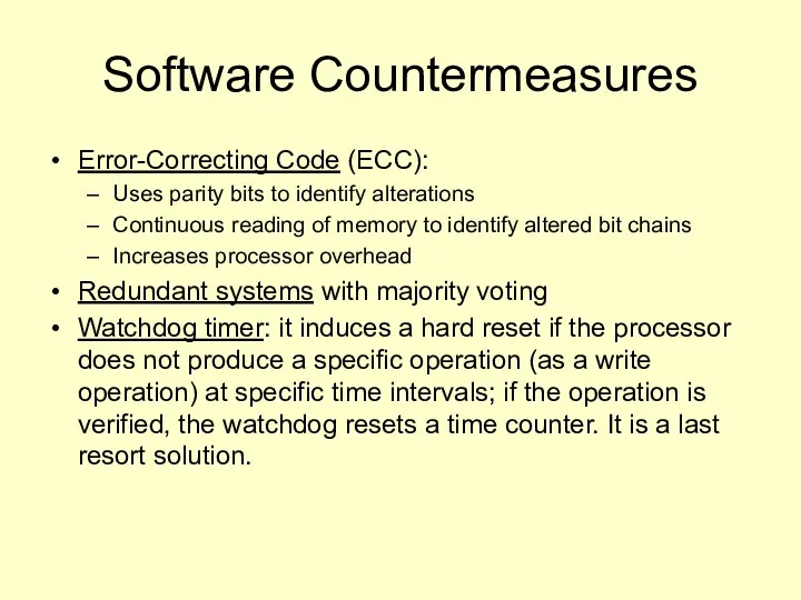
Software Countermeasures
Error-Correcting Code (ECC):
Uses parity bits to identify alterations
Continuous reading of
Software Countermeasures
Error-Correcting Code (ECC):
Uses parity bits to identify alterations
Continuous reading of
Micrometeoroids (1)
Micrometeoroids (and space debris) do not usually destroy a satellite,
Micrometeoroids (1)
Micrometeoroids (and space debris) do not usually destroy a satellite,
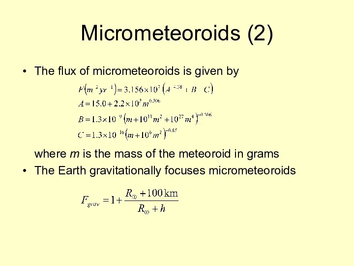
Micrometeoroids (2)
The flux of micrometeoroids is given by
where m is the
Micrometeoroids (2)
The flux of micrometeoroids is given by
where m is the
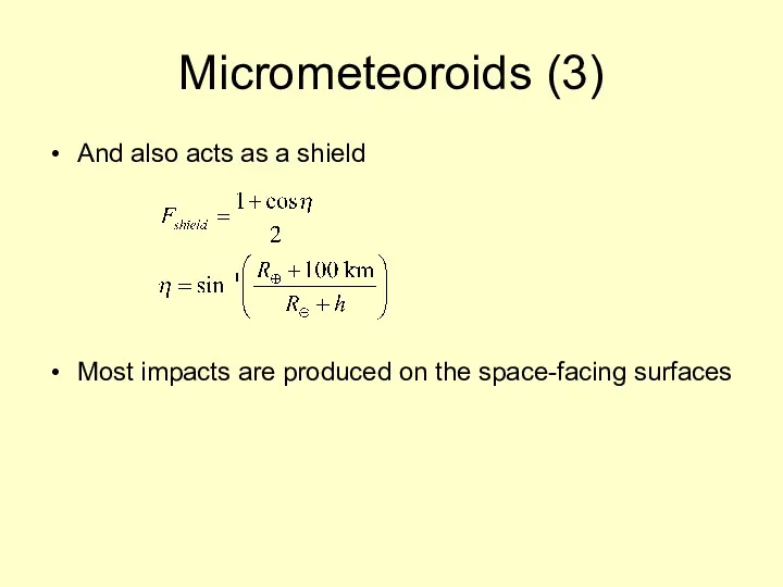
Micrometeoroids (3)
And also acts as a shield
Most impacts are produced on
Micrometeoroids (3)
And also acts as a shield
Most impacts are produced on
Gravitational focusing
Planetary shielding
Gravitational focusing
Planetary shielding
Space debris (1)
Space debris are produced by human activities in space
They
Space debris (1)
Space debris are produced by human activities in space
They
Space debris (2)
Space debris at heights of less than 600 km
Space debris (2)
Space debris at heights of less than 600 km
Kessler syndrome
It is possible that a series of collisions between space
Kessler syndrome
It is possible that a series of collisions between space
Our swarm as a space debris hazard
A large swarm could be
Our swarm as a space debris hazard
A large swarm could be
Debris Mitigation
The United Nations, through its Office for Outer Space Affairs,
Debris Mitigation
The United Nations, through its Office for Outer Space Affairs,
References
General references
Alan C. Tribble, The Space Environment, Princeton University Press (2003)
Vincent
References
General references
Alan C. Tribble, The Space Environment, Princeton University Press (2003)
Vincent
References
Atomic Oxygen Erosion
Zhan, Y., & Zhang, G., Low Earth orbit environmental
References
Atomic Oxygen Erosion
Zhan, Y., & Zhang, G., Low Earth orbit environmental
 Закони і формули в астрономії
 Физика Солнца
 Планета Сатурн
 Малые тела Солнечной системы
 Закони і формули астрономії
 Астероидная опасность - миф или реальность
 Казка зоряного неба
 Луна
Луна Марс. Несколько интересных фактов
 Сенсоры и платформы дистанционного зондирования Земли из космоса
 Пути реализации задачи организации связи с объектами, расположенными на орбите и поверхности планет Солнечной системы
 Надежда. Новая надежда человечества
 Созвездия Лебедь и Лира
 Проект для детей 5-6 лет Большое космическое путешествие
 Дошкольникам о космосе
 Interesting facts about space
 Спектры, цвет и температура звёзд
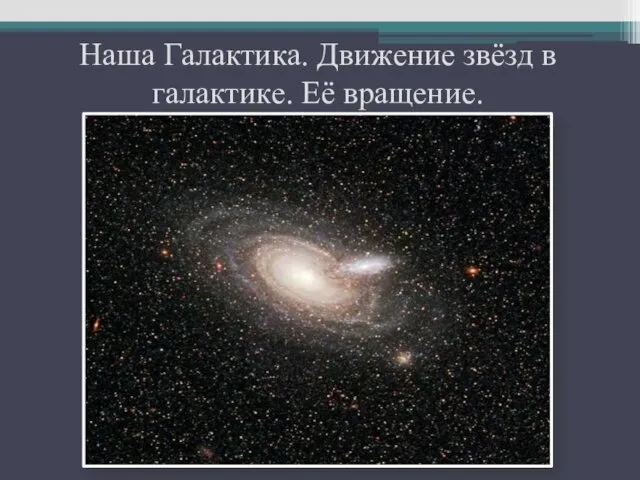 Наша Галактика. Движение звёзд в галактике. Её вращение
 Определение расстояний и размеров тел в Солнечной системе
 Галактики. Виды галактик во Вселеной
 Планета Земля
 Современное состояние и перспективы развития аэрокосмической техники. Малая космонавтика
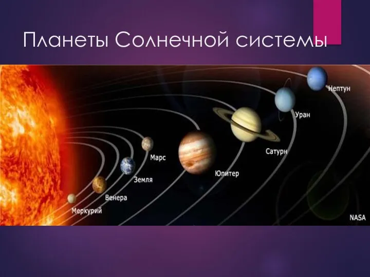 Планеты Солнечной системы
 Фазы Луны. Лунное затмение
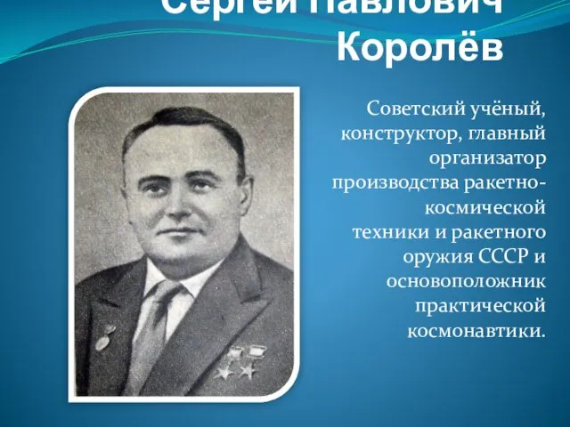 Сергей Павлович Королёв
 Строение Земли
 Обсерваторії. Орбітальна обсерваторія NASA
 Переменные звёзды. Двойные звёзды. Движение звёзд