- Lecture # 09. Inputs and Production Functions

Содержание
- 2. Outline The Production Function Marginal and Average Products Isoquants Marginal Rate of Technical Substitution Returns to
- 3. Definitions Inputs or factors of production are productive resources that firms use to manufacture goods and
- 4. Definitions Production transforms a set of inputs into a set of outputs Technology determines the quantity
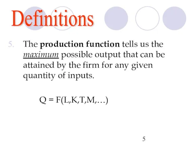
- 5. Definitions The production function tells us the maximum possible output that can be attained by the
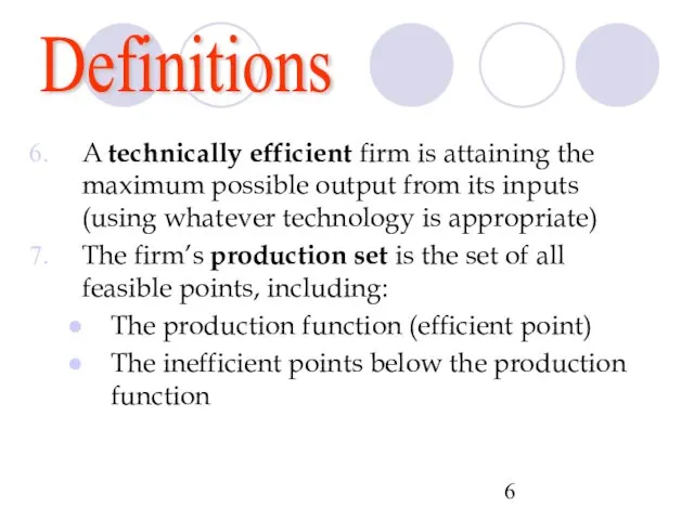
- 6. Definitions A technically efficient firm is attaining the maximum possible output from its inputs (using whatever
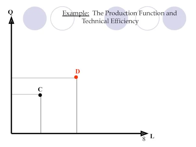
- 7. Example: The Production Function and Technical Efficiency L Q • C
- 8. Example: The Production Function and Technical Efficiency L Q • • C D
- 9. Example: The Production Function and Technical Efficiency Q = f(L) L Q • • C D
- 10. Example: The Production Function and Technical Efficiency Q = f(L) L Q • • • •
- 11. Example: The Production Function and Technical Efficiency Q = f(L) L Q • • • •
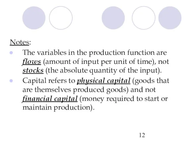
- 12. Notes: The variables in the production function are flows (amount of input per unit of time),
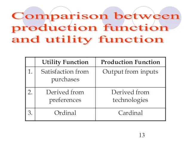
- 13. Comparison between production function and utility function
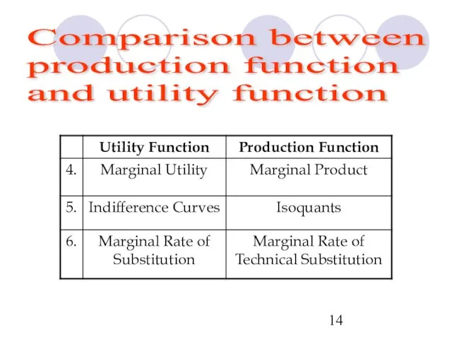
- 14. Comparison between production function and utility function
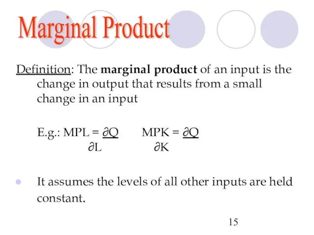
- 15. Marginal Product Definition: The marginal product of an input is the change in output that results
- 16. Example: Suppose Q = K0.5L0.5 Then: MPL = ∂Q = 0.5 K0.5 ∂L L0.5 MPK =
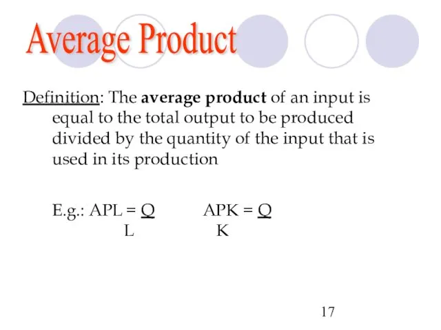
- 17. Average Product Definition: The average product of an input is equal to the total output to
- 18. Example: Suppose Q = K0.5L0.5 Then: APL = Q = K0.5L0.5 = K0.5 L L L0.5
- 19. Law of Diminishing Marginal Returns Definition: The law of diminishing marginal returns states that the marginal
- 20. Q L Q= F(L,K0) Example: Total and Marginal Product
- 21. Q L MPL maximized Q= F(L,K0) Example: Total and Marginal Product Increasing marginal returns Diminishing marginal
- 22. Q L MPL = 0 when TP maximized Q= F(L,K0) Example: Total and Marginal Product Diminishing
- 23. Example: Total and Marginal Product L MPL Q L MPL maximized TPL maximized where MPL is
- 24. Marginal and Average Products There is a systematic relationship between average product and marginal product. This
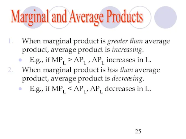
- 25. Marginal and Average Products When marginal product is greater than average product, average product is increasing.
- 26. Example: Average and Marginal Products L APL MPL MPL maximized APL maximized
- 27. Example: Total, Average and Marginal Products L APL MPL Q L MPL maximized APL maximized
- 28. Isoquants Definition: An isoquant is a representation of all the combinations of inputs (labor and capital)
- 29. Example: Isoquants L K Q = 10 0 Slope=dK/dL L
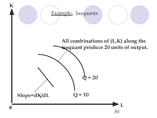
- 30. L Q = 10 Q = 20 All combinations of (L,K) along the isoquant produce 20
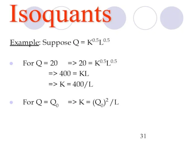
- 31. Isoquants Example: Suppose Q = K0.5L0.5 For Q = 20 => 20 = K0.5L0.5 => 400
- 32. Definition: The marginal rate of technical substitution measures the rate at which the firm can substitute
- 33. Marginal Rate Of Technical Substitution Alternative Definition : It is the negative of the slope of
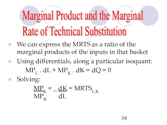
- 34. Marginal Product and the Marginal Rate of Technical Substitution We can express the MRTS as a
- 35. Marginal Product and the Marginal Rate of Technical Substitution Notes: If we have diminishing marginal returns,
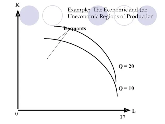
- 36. Marginal Product and the Marginal Rate of Technical Substitution Notes: If both marginal products are positive,
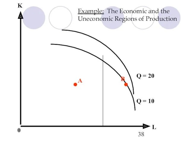
- 37. Example: The Economic and the Uneconomic Regions of Production L K Q = 10 Q =
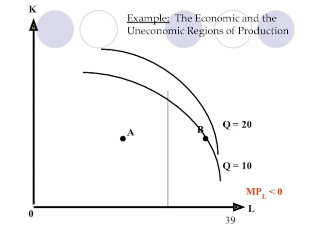
- 38. Example: The Economic and the Uneconomic Regions of Production L K Q = 10 Q =
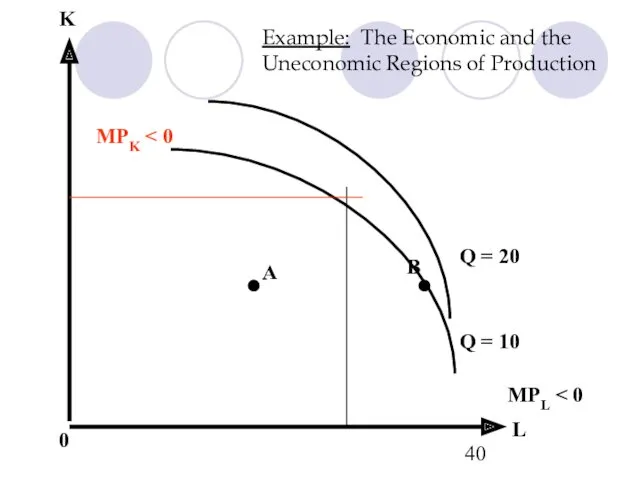
- 39. Example: The Economic and the Uneconomic Regions of Production L K Q = 10 Q =
- 40. Example: The Economic and the Uneconomic Regions of Production L K Q = 10 Q =
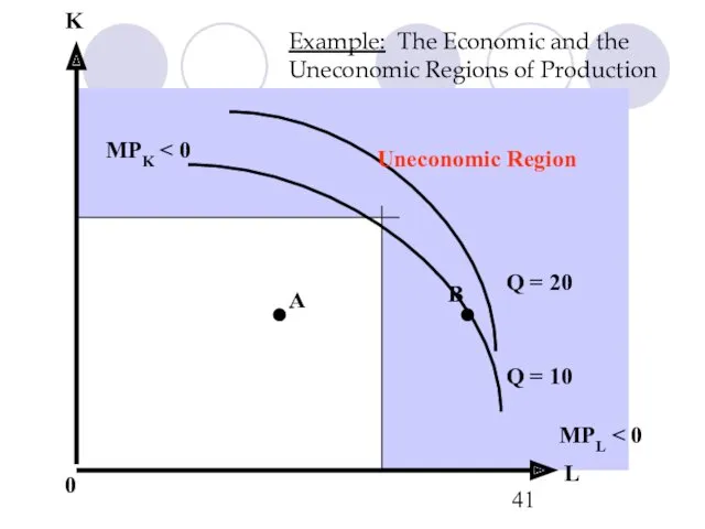
- 41. Example: The Economic and the Uneconomic Regions of Production L K Q = 10 Q =
- 43. Скачать презентацию
Outline
The Production Function
Marginal and Average Products
Isoquants
Marginal Rate of Technical Substitution
Returns to
Outline
The Production Function
Marginal and Average Products
Isoquants
Marginal Rate of Technical Substitution
Returns to

Definitions
Inputs or factors of production are productive resources that firms use
Definitions
Inputs or factors of production are productive resources that firms use

Definitions
Production transforms a set of inputs into a set of outputs
Technology
Definitions
Production transforms a set of inputs into a set of outputs
Technology
Definitions
The production function tells us the maximum possible output that can
Definitions
The production function tells us the maximum possible output that can
Definitions
A technically efficient firm is attaining the maximum possible output from
Definitions
A technically efficient firm is attaining the maximum possible output from
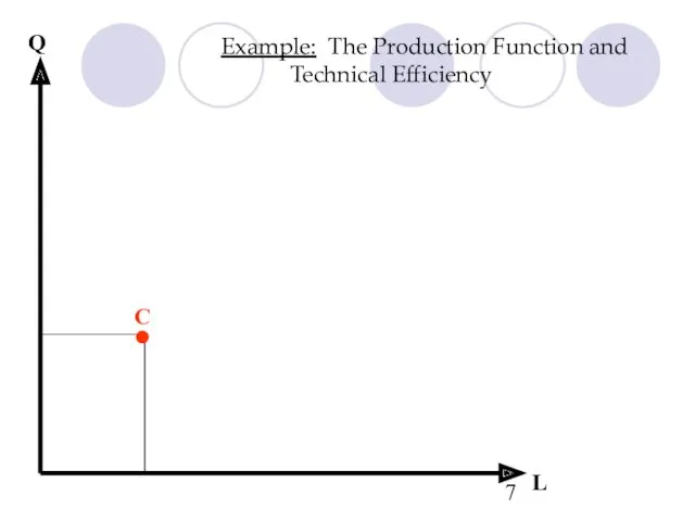
Example: The Production Function and Technical Efficiency
L
Q
•
C
Example: The Production Function and Technical Efficiency
L
Q
•
C
Example: The Production Function and Technical Efficiency
L
Q
•
•
C
D
Example: The Production Function and Technical Efficiency
L
Q
•
•
C
D
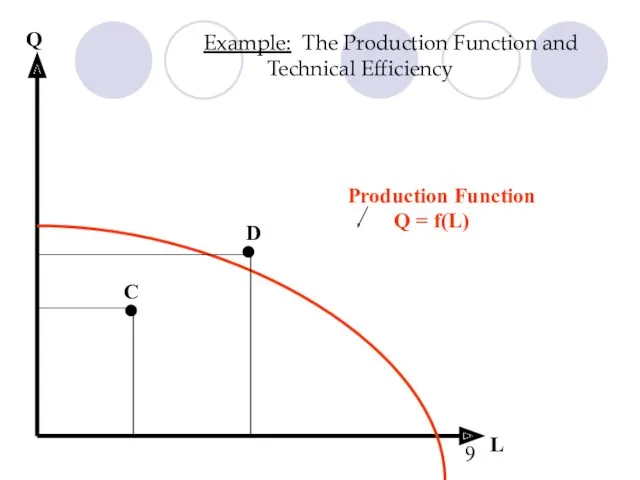
Example: The Production Function and Technical Efficiency
Q = f(L)
L
Q
•
•
C
D
Production Function
Example: The Production Function and Technical Efficiency
Q = f(L)
L
Q
•
•
C
D
Production Function
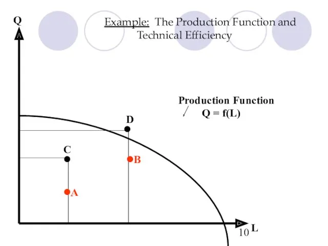
Example: The Production Function and Technical Efficiency
Q = f(L)
L
Q
•
•
•
•
C
D
A
B
Production Function
Example: The Production Function and Technical Efficiency
Q = f(L)
L
Q
•
•
•
•
C
D
A
B
Production Function
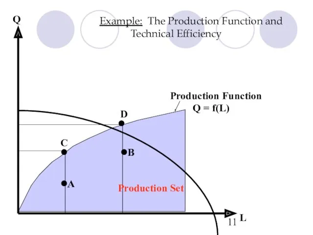
Example: The Production Function and Technical Efficiency
Q = f(L)
L
Q
•
•
•
•
C
D
A
B
Production Set
Production
Example: The Production Function and Technical Efficiency
Q = f(L)
L
Q
•
•
•
•
C
D
A
B
Production Set
Production
Notes:
The variables in the production function are flows (amount of input
Notes:
The variables in the production function are flows (amount of input
Comparison between
production function
and utility function
Comparison between
production function
and utility function
Comparison between
production function
and utility function
Comparison between
production function
and utility function
Marginal Product
Definition: The marginal product of an input is the change
Marginal Product
Definition: The marginal product of an input is the change
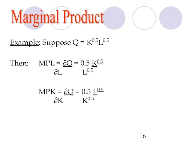
Example: Suppose Q = K0.5L0.5
Then: MPL = ∂Q = 0.5 K0.5
Example: Suppose Q = K0.5L0.5
Then: MPL = ∂Q = 0.5 K0.5
Average Product
Definition: The average product of an input is equal to
Average Product
Definition: The average product of an input is equal to
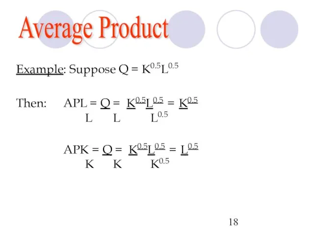
Example: Suppose Q = K0.5L0.5
Then: APL = Q = K0.5L0.5 =
Example: Suppose Q = K0.5L0.5
Then: APL = Q = K0.5L0.5 =
Law of Diminishing Marginal Returns
Definition: The law of diminishing marginal returns
Law of Diminishing Marginal Returns
Definition: The law of diminishing marginal returns
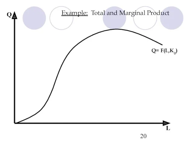
Q
L
Q= F(L,K0)
Example: Total and Marginal Product
Q
L
Q= F(L,K0)
Example: Total and Marginal Product

Q
L
MPL maximized
Q= F(L,K0)
Example: Total and Marginal Product
Increasing marginal returns
Diminishing marginal returns
Q
L
MPL maximized
Q= F(L,K0)
Example: Total and Marginal Product
Increasing marginal returns
Diminishing marginal returns
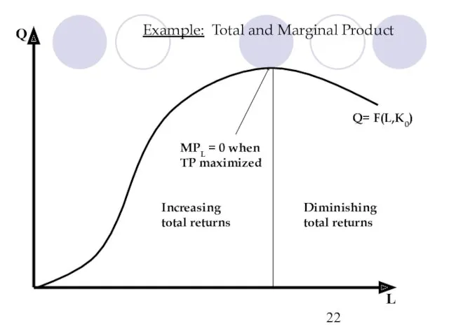
Q
L
MPL = 0 when
TP maximized
Q= F(L,K0)
Example: Total and Marginal Product
Diminishing total
Q
L
MPL = 0 when
TP maximized
Q= F(L,K0)
Example: Total and Marginal Product
Diminishing total
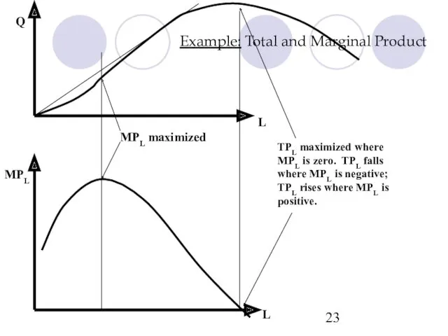
Example: Total and Marginal Product
L
MPL
Q
L
MPL maximized
TPL maximized where
MPL is zero. TPL
Example: Total and Marginal Product
L
MPL
Q
L
MPL maximized
TPL maximized where
MPL is zero. TPL
Marginal and Average Products
There is a systematic relationship between average product
Marginal and Average Products
There is a systematic relationship between average product
Marginal and Average Products
When marginal product is greater than average product,
Marginal and Average Products
When marginal product is greater than average product,

Example: Average and Marginal Products
L
APL
MPL
MPL maximized
APL maximized
Example: Average and Marginal Products
L
APL
MPL
MPL maximized
APL maximized
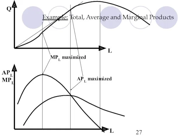
Example: Total, Average and Marginal Products
L
APL
MPL
Q
L
MPL maximized
APL maximized
Example: Total, Average and Marginal Products
L
APL
MPL
Q
L
MPL maximized
APL maximized
Isoquants
Definition: An isoquant is a representation of all the combinations of
Isoquants
Definition: An isoquant is a representation of all the combinations of
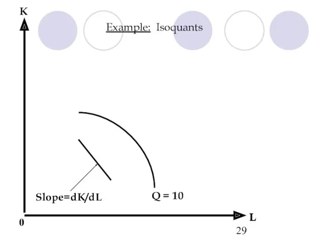
Example: Isoquants
L
K
Q = 10
0
Slope=dK/dL
L
Example: Isoquants
L
K
Q = 10
0
Slope=dK/dL
L
L
Q = 10
Q = 20
All combinations of (L,K) along the
isoquant produce
L
Q = 10
Q = 20
All combinations of (L,K) along the
isoquant produce
Isoquants
Example: Suppose Q = K0.5L0.5
For Q = 20 => 20 =
Isoquants
Example: Suppose Q = K0.5L0.5
For Q = 20 => 20 =
Definition: The marginal rate of technical substitution measures the rate at
Definition: The marginal rate of technical substitution measures the rate at
Marginal Rate Of Technical Substitution
Alternative Definition : It is the
Marginal Rate Of Technical Substitution
Alternative Definition : It is the
Marginal Product and the Marginal
Rate of Technical Substitution
We can
Marginal Product and the Marginal
Rate of Technical Substitution
We can
Marginal Product and the Marginal
Rate of Technical Substitution
Notes:
If we
Marginal Product and the Marginal
Rate of Technical Substitution
Notes:
If we
Marginal Product and the Marginal
Rate of Technical Substitution
Notes:
If both
Marginal Product and the Marginal
Rate of Technical Substitution
Notes:
If both
Example: The Economic and the Uneconomic Regions of Production
L
K
Q =
Example: The Economic and the Uneconomic Regions of Production
L
K
Q =
Example: The Economic and the Uneconomic Regions of Production
L
K
Q =
Example: The Economic and the Uneconomic Regions of Production
L
K
Q =
Example: The Economic and the Uneconomic Regions of Production
L
K
Q =
Example: The Economic and the Uneconomic Regions of Production
L
K
Q =
Example: The Economic and the Uneconomic Regions of Production
L
K
Q =
Example: The Economic and the Uneconomic Regions of Production
L
K
Q =
Example: The Economic and the Uneconomic Regions of Production
L
K
Q =
Example: The Economic and the Uneconomic Regions of Production
L
K
Q =
 經濟學無路用?! 外匯保證金投資 輔 大 經 濟 系
 Теория Мальтуса
 Социальные нормы и их роль в экономике
 Торгово-экономическое сотрудничество ЕАЭС и КНР
 Безработица. Причины безработицы
 Дипломдық жоба
 Международная компания
 О мерах поддержки, предоставляемых но Фонд развития моногородов
 Нарықтық экономиканың жалпы сипаттамасы
 Кафедра устойчивого инновационного развития. Системный анализ и управление устойчивым развитием сложных систем. Лекции
 Рыночные отношения в экономике. Тема 3.2
 Цена - это денежное выражение стоимости товаров и услуг
 Свободные экономические зоны в мировой экономике Филиппины и Тайланд
 Бюджет семьи и бережное потребление
 Макроэкономическое равновесие. Классический и кейнсианский подход
 Типы условий оптимизации развития ЭЭС. Критерии принятия решений в условиях неопределенности
 Государство и рынок. Модуль 6. Часть 1
 Совершенная и несовершенная конкуренция. Тема 7
 Роль грошей у ринковій економіці
 Public Goods and Common Resource
 Тема 9. Рынок земли
 Экономическое регулирование автомобильных перевозок
 Теория ценности, капитала и земельной ренты. Давид Рикардо (1772-1823)
 Интернациональная система качественного развития ИСКР.РФ
 Презентація з економіки до теми Сімейний бюджет
 Організація наукових досліджень у США
 Рыночная конкуренция. (Тема 6)
 Исландия экономикасы