- Lecture 8. Basics of time series. Forecasting

Содержание
- 2. LECTURE 8 BASICS OF TIME SERIES. FORECASTING Temur Makhkamov Indira Khadjieva QM Module Leader Room IB
- 3. Lecture outline: to estimate the change of a value over time and graph the dynamics of
- 4. Components of time series graph Trend – the overall pattern of changes in a specific value
- 5. Additive Model
- 6. Multiplicative Model
- 7. Case 1: quarterly computer sales
- 8. Graphical representation Time series graph
- 9. Additive model (1) Draw the trend line using the equation function (Trend) Subtract trend (CMA) value
- 10. Additive model (2) Forecasted trendline
- 11. Additive model (3)
- 12. Additive model (4)
- 13. Additive model (5) Average of average deviations Average deviations minus Adjustment
- 14. Additive model (6)
- 15. Multiplicative model (1) Draw the trend line using the equation function (Trend) Divide the actual value
- 16. Multiplicative model (2)
- 17. Multiplicative model (3) Average of average deviations Average deviations divided by Adjustment
- 18. Multiplicative model (4) Trend line for the 4th quarter of 2021 indicates that the value equals
- 19. Concluding remarks Today, you learnt Graphical display of the change of a value over time Time
- 21. Скачать презентацию

LECTURE 8
BASICS OF TIME SERIES. FORECASTING
Temur Makhkamov
Indira Khadjieva
QM Module Leader
Room
LECTURE 8
BASICS OF TIME SERIES. FORECASTING
Temur Makhkamov
Indira Khadjieva
QM Module Leader
Room

Lecture outline:
to estimate the change of a value over time and
Lecture outline:
to estimate the change of a value over time and

Components of time series graph
Trend – the overall pattern of changes
Components of time series graph
Trend – the overall pattern of changes

Additive Model
Additive Model

Multiplicative Model
Multiplicative Model

Case 1: quarterly computer sales
Case 1: quarterly computer sales

Graphical representation
Time series
graph
Graphical representation
Time series
graph

Additive model (1)
Draw the trend line using the equation function (Trend)
Subtract
Additive model (1)
Draw the trend line using the equation function (Trend)
Subtract

Additive model (2)
Forecasted trendline
Additive model (2)
Forecasted trendline

Additive model (3)
Additive model (3)

Additive model (4)
Additive model (4)

Additive model (5)
Average of average deviations
Average deviations minus Adjustment
Additive model (5)
Average of average deviations
Average deviations minus Adjustment

Additive model (6)
Additive model (6)

Multiplicative model (1)
Draw the trend line using the equation function (Trend)
Divide
Multiplicative model (1)
Draw the trend line using the equation function (Trend)
Divide

Multiplicative model (2)
Multiplicative model (2)

Multiplicative model (3)
Average of average deviations
Average deviations divided by Adjustment
Multiplicative model (3)
Average of average deviations
Average deviations divided by Adjustment

Multiplicative model (4)
Trend line for the 4th quarter of 2021 indicates
Multiplicative model (4)
Trend line for the 4th quarter of 2021 indicates

Concluding remarks
Today, you learnt
Graphical display of the change of a value
Concluding remarks
Today, you learnt
Graphical display of the change of a value
 Чистый обмен и основы разделения труда. Лекция 5
 Предложение на рынке с совершенной конкуренцией
 Информация, неопределенность, риск в экономике
 Агломерации и их эффекты
 Денежная система
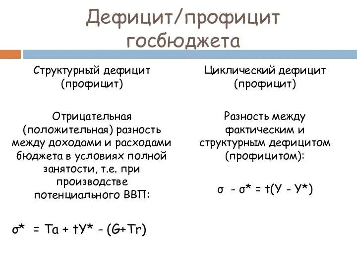 Дефицит/профицит госбюджета
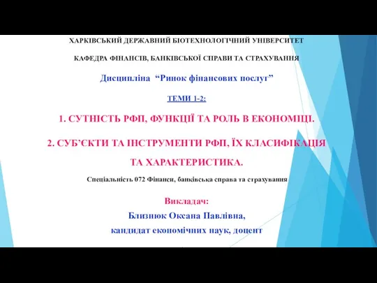 Сутність РФП, функції та роль в економіці. Суб’єкти та інструменти РФП, їх класифікація та характеристика. Теми 1-2
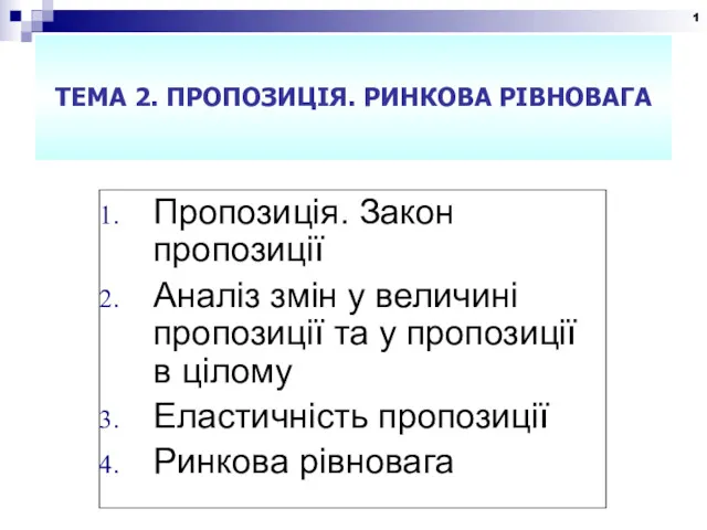 Пропозиція. Ринкова рівновага
 Политико-экономические механизмы функционирования сектора государственного управления. Лекция 11
 Обмен, торговля, реклама
 Public Goods and Common Resource
 Экономика. Искусство ведения хозяйства
 Функции государства в экономике
 Цивилізаційні виміри глобальних виробничих процесів
 Казахстанская модель экономического развития
 Функционально-стоимостной анализ
 План продаж 2016 Алтех .Техника для обработки почвы
 Кадастровая стоимость и нормативная цена земли
 Экономика родного края
 Формирование политики доходов населения в Монако
 Предпринимательство как фактор производства
 Индия в системе современных международных отношений
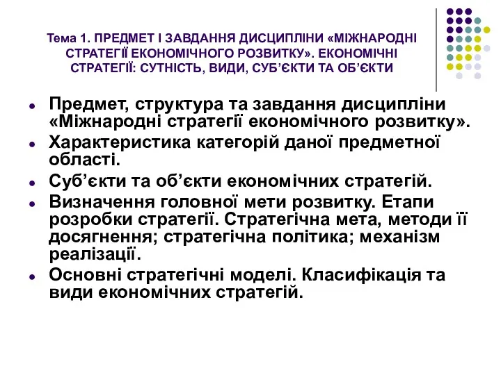 Міжнародні стратегії економічного розвитку. Економічні стратегії, сутність та види
 Экономические реформы П.А.Столыпина
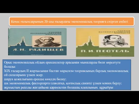 Кеңес ғалымдарының 20-шы ғасырдағы экономикалық теорияға сңірген еңбегі
 Своя игра по экономике
 География основных типов экономики на территории России
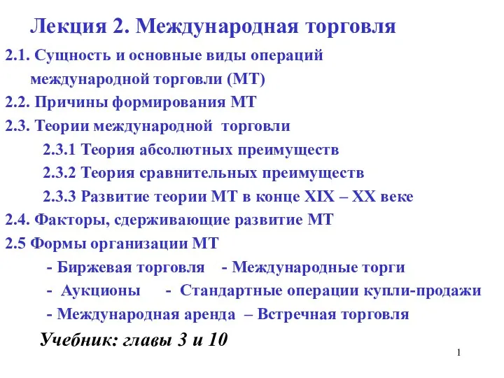 Международная торговля