- Reservoir management

Содержание
- 2. Learning objectives Provide a formal Management Process Reservoir Management tools Review some examples of Management Strategy
- 3. “The purpose of reservoir management is to control operations to obtain the maximum possible economic recovery
- 4. “The marshalling of all appropriate business, technical and operating resources to exploit a reservoir optimally from
- 5. “There are probably as many different definitions as there are perceptions of the process” “Integrated approach...key
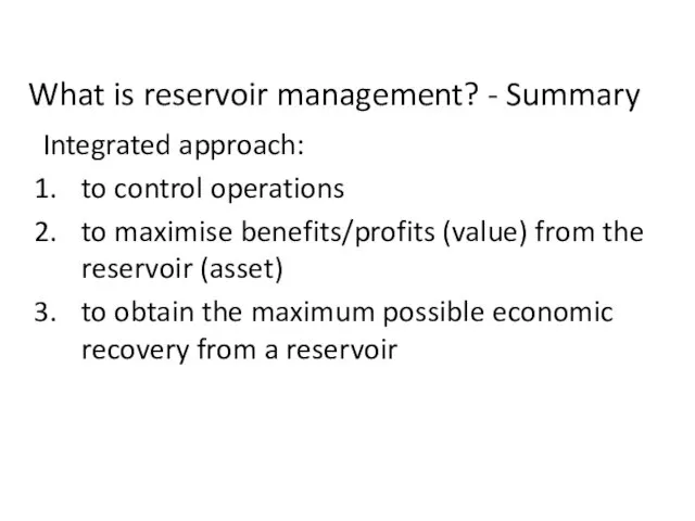
- 6. What is reservoir management? - Summary Integrated approach: to control operations to maximise benefits/profits (value) from
- 7. A lifetime of reservoir models
- 8. Forties field – habitat of remaining oil (from Brand et al., 1996; Scott, 1997)
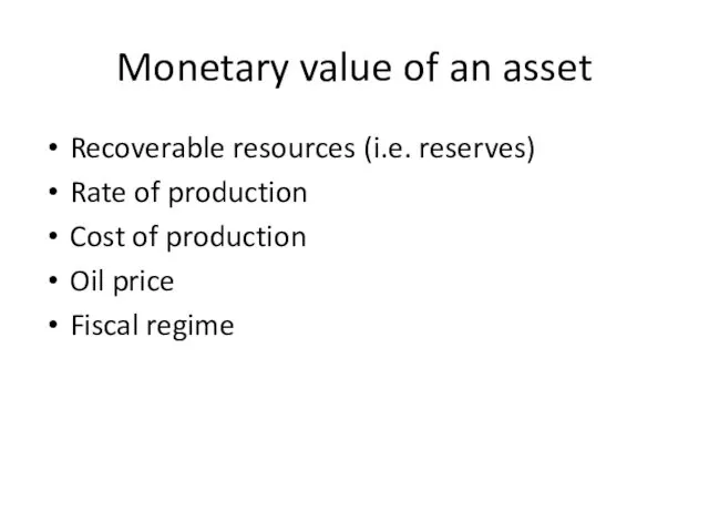
- 9. Monetary value of an asset Recoverable resources (i.e. reserves) Rate of production Cost of production Oil
- 10. Aim MAXIMISE VALUE MINIMISE COST Maximise recovery Recovery Technology (speed up) People/Team Reservoir Knowledge/analysis CAPEX OPEX
- 11. RECOVERY Maximise value through…
- 12. Recovery Factors Tyler and Finlay, 1991 Depends on Geology and Drive Mechanism Solution gas drive 5-30%
- 13. Depositional Environment vs Drive Mechanism Environment type has less of an impact on recovery efficiency Primary
- 14. Recover efficiency impact from various reservoir features
- 15. Does connectivity influence recovery?
- 16. What is connectivity? Sandbody connectivity % of sand bodies that are connected to each other Reservoir
- 17. Examples of connectivity? Larue & Hovadik, 2006
- 18. Relationship between connectivity and recovery Larue & Hovadik, 2006
- 19. Static vs dynamic well connectivity Reservoir recoveries significantly below percolation prediction of connected sand bodies Static
- 20. 2D Connectivity Hovadik & Larue, 2010
- 21. 3D percolation connectivity Hovadik & Larue, 2010
- 22. 2D vs 3D connectivity Larue & Hovadik, 2006
- 23. Shifting the S-Curve Larue & Hovadik, 2006
- 24. Shifting the S-Curve Left or Right? 1 2 3 6 7 8 5 4 Larue &
- 25. Geology that shifts the S-Curve Left Larue & Hovadik, 2006
- 26. Geology that shifts the S-Curve Right Larue & Hovadik, 2006
- 27. Increasing 2D effect (shift to Right) Larue & Hovadik, 2006
- 28. Volume support and the cascade zone Larue & Hovadik, 2006
- 29. Geobody Anisotropy Hovadik & Larue, 2010
- 30. Sinuosity Hovadik & Larue, 2010
- 31. Grid dimensions – volume support Hovadik & Larue, 2007/2010
- 32. Overview Increased volume support increases width of cascade zone Decreasing “dimensionality” moves curve to right Increasing
- 33. Which impact? X X X X X X X X X X X X X
- 34. Is connectivity the biggest factor affecting recovery? Larue and Friedman, 2005
- 35. 30% NTG Larue and Friedman, 2005
- 36. 60% NTG Larue and Friedman, 2005
- 37. 80% NTG Larue and Friedman, 2005
- 38. Key factors affecting dynamic recovery Static connectivity SHAPE OF S-CURVE Dynamic “addons” Tortuosity Permeability Heterogeneity Inter-well
- 39. Impact of tortuosity Larue & Hovadik, 2006
- 40. Impact of permeability heterogeneity Larue and Friedman, 2005
- 41. Thief zone impact on recovery Larue and Friedman, 2005
- 42. Permeabilty heterogeneity impact Small difference between 0D (nugget) and 3D (variogram) models Add trend to increase
- 43. Variogram range and Vdp combined Hovadik & Larue, 2010
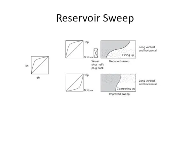
- 44. Reservoir Sweep
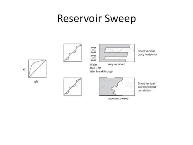
- 45. Reservoir Sweep
- 46. Reservoir Sweep
- 47. Impact of mobility ratio Larue and Friedman, 2005
- 48. Impact of well pattern Larue and Friedman, 2005
- 49. Well distance impact on recovery (dynamic connectivity) Hovadik & Larue, 2010
- 50. Does seed really account for uncertainty? Larue and Friedman, 2005
- 51. What matters in your reservoir? Larue and Friedman, 2005
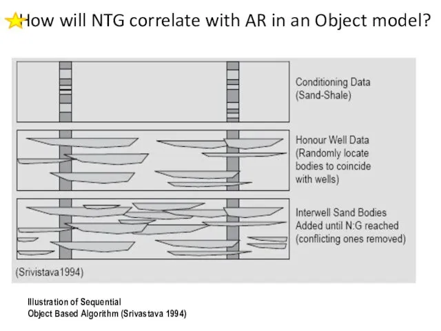
- 52. Extreme edge cases: High NTG + Low Connectivity Manzocchi et al, 2007
- 53. NTG vs Amalgamation Ratio NTG and Amalgamation ratio do not corellate in real systems (e.g. turbidites)
- 54. Object Based Modelling Convergence Problem Illustration of Sequential Object Based Algorithm (Srivastava 1994) As Number of
- 55. Geostatistical modelling conditioned to NTG High NTG system has short continuity of sandbodies vertically and laterally
- 56. Overview of connectivity 30% 60% A+B NTG NTG Geobody size Total Recovery Impact of Geology More
- 57. IMPROVED RECOVERY Maximise value through…
- 58. Recovery Factors Tyler and Finlay, 1991 Depends on Geology and Drive Mechanism Solution gas drive 5-30%
- 59. Improved Recover Factors Tyler and Finlay, 1991
- 60. What can we adjust to improve recovery?
- 61. Evaluation of history, IHS data base Natural decline “as is” Production efficiency Reserve growth; IOR and
- 62. Production Capacity Increase in Mature Fields Time Production Overall Field Development Plan Detailed Seismic & Geology
- 63. Production Capacity Increase in Mature Fields Time Production Overall Field Development Plan Detailed Seismic & Geology
- 64. INFILL DRILLING Example of….
- 65. Time Field Oil Production Rate A typical example of the north sea
- 66. RM Example 1 Strategy for Statfjord Aadland et al., 1994 High well activity Horizontal wells Reservoir
- 67. Statfjord Field - cross section GOC OWC GOC OWC BRENT STATFJORD 200m
- 68. Statfjord Field - initial production plan BRENT STATFJORD 200m Water injection Gas injection Oil production
- 69. Statfjord Field - Remaining oil BRENT STATFJORD 200m Remaining oil locations Rim oil Attic oil Structural
- 70. Statfjord Field - New opportunities BRENT STATFJORD 200m Remaining oil locations New completions Horizontal wells High
- 71. Example: Yibal Field, Oman Strategy for Yibal Field, Oman Horizontal wells Bypassed oil in a Carbonate
- 72. Modelling Characteristics and Sensitivities Original OWC Upper Shuaiba Matrix: Single pore system Uncertain Kv/Kh ratio Uncertain
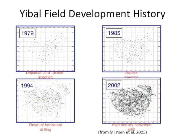
- 73. Yibal Field Development History Depletion and “phase” injection Aquifer injection Onset of horizontal drilling High density
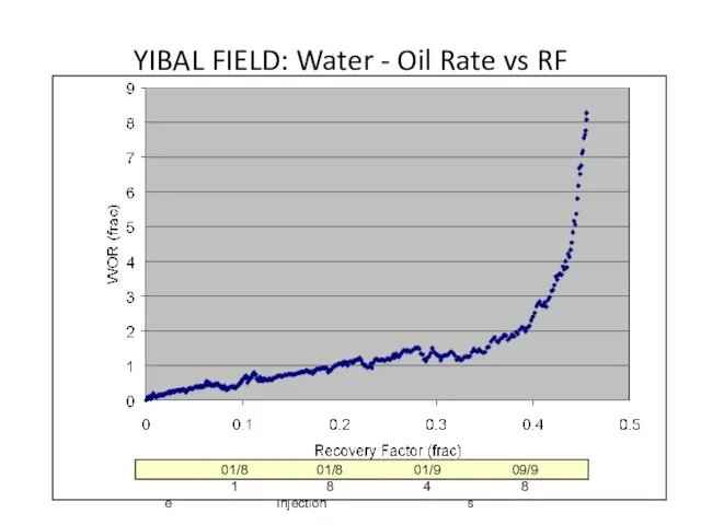
- 74. YIBAL FIELD: Water - Oil Rate vs RF Phase Aquifer Injection Horizontals 01/81 01/88 01/94 09/98
- 75. Seifert et al., 1996 Impact of well placement fluvial study SW NE compartmentalisation of pay facies
- 76. Seifert et al., 1996 Impact of well placement fluvial study find orientation of well trajectory most
- 77. Seifert et al., 1996 Impact of well placement results aeolian bodies intersected aeolian GU proportions horizontal
- 78. RM Example 3: Heather Field Compartmentalisation and Variable Recovery Crest Flank
- 79. Infill Drilling – Heather Field Fault compartmentalisation
- 80. FRACCING Example of….
- 81. Example: Leman Field Strategy for Leman Field Mijnsson and Maskall 1994 Proactive hunt for gas Horizontal
- 82. Typical Rotliegend reservoir section
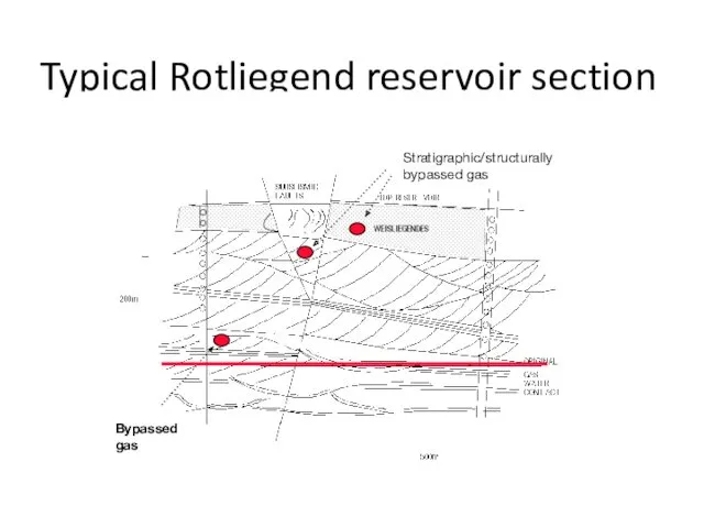
- 83. Typical Rotliegend reservoir section Bypassed gas Stratigraphic/structurally bypassed gas
- 84. Typical Rotliegend reservoir section Horizontal well/multilateral opportunities Stratigraphic/structurally bypassed gas Fraccing
- 85. EOR (WAG) Example of….
- 86. IOR: New opportunities with CO2 Initial Waterflood Main CO2 flood ROZ CO2 flood mbd
- 87. Example: Magnus Field Production & Injection History Commence water injection Moulds et al, 2010, SPE 134953
- 88. Improved oil recovery from EOR over waterflood Moulds et al, 2010, SPE 134953
- 89. The Future – New Wells Magnus Extension Project 4 new slots, slot splitter technology enables 2
- 90. Target: Magnus Field Oil Remaining after waterflood EOR oil target: updip attic target and unswept oil
- 91. PEOPLE/TEAMS Maximise value through…
- 92. Synergy Output of a synergistic team is larger than the sum of the output of individuals….
- 93. Synergy Is not: Geoengineering Any thing about multi-discipline work Anything to do with Energy Synergy Sum
- 94. REM is like Systems thinking System of interdependent processes Model Complexity of system rather than simplify
- 95. Field Management Plan (UK DTI) Reservoir Management Strategy - detailing the principles and objectives that the
- 96. RM Strategy Developing Implementing Monitoring Evaluating DIME - Satter and Thakur, 1994
- 97. WATER MANAGEMENT Increase costs through…
- 98. Reservoir Management Issues (1) a- Mechanical leaks: b - Behind Casing flow c - Oil-water contact:
- 99. Reservoir Management Issues (2) e- Fractures: f – Fractures to water g - Coning: h –
- 100. WATER SHUTOFF Example of….
- 101. Yibal Field Development History Depletion and “phase” injection Aquifer injection Onset of horizontal drilling High density
- 102. YIBAL FIELD: Water - Oil Rate vs RF Phase Aquifer Injection Horizontals 01/81 01/88 01/94 09/98
- 103. Brent Field Reservoir monitoring (Bryant and Livera, 1991)
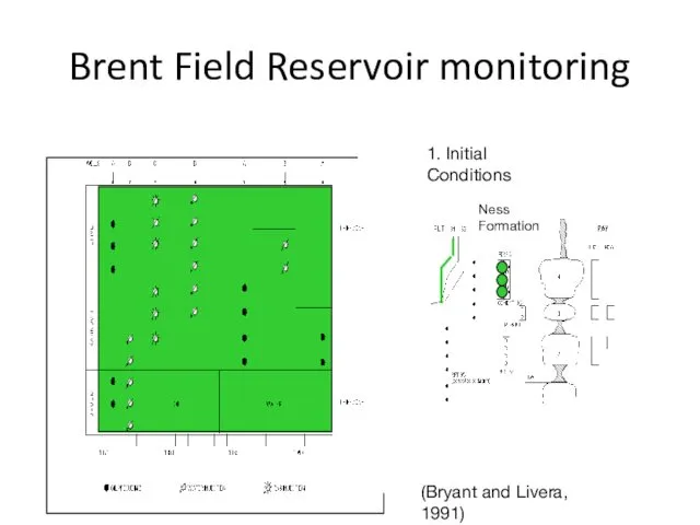
- 104. Brent Field Reservoir monitoring (Bryant and Livera, 1991) 1. Initial Conditions Ness Formation
- 105. Brent Field Reservoir monitoring (Bryant and Livera, 1991) 1. 1987 Conditions Ness Formation New Perforations Profile
- 106. SCALE MANAGEMENT Increase costs through…
- 107. Decline in Magnus production Moulds et al, 2010, SPE 134953
- 108. Examples - Flow Restriction
- 109. Examples - Facilities separator scaled up and after cleaning
- 110. Water chemistry history match 154471 • Use of Water Chemistry Data in History Matching of a
- 111. Probabilistic predictions of scaling in wells 154471 • Use of Water Chemistry Data in History Matching
- 112. Predicting Seawater fraction in produced water (Vasquez et al., 2013)
- 113. Probability maps of seawater fraction P10 P50 P90
- 114. Results Optimization w/o accounting scale risk
- 115. Results Optimization accounting scale risk SeaWater Fraction OilSaturation Layer 4 OilSaturation Layer 1
- 116. Results Layer open/shut w/o accounting scale risk accounting scale risk 0 1
- 117. Impact in the value through… VALUE OF YOUR OIL
- 118. Two key things you don’t know How much oil you can extract Reservoir uncertainty Variations from
- 119. All oil is not created equally priced...
- 120. Time value of money where DPV is the discounted present value of the future cash flow
- 121. Value of money decreases overtime (NPV) From wikipedia
- 122. Compare value of companies Oil = 5,817 million barrels Gas = 24,948 billion cubic feet 1.75
- 123. Compare strategy of companies Offshore, deep water, complex fields Ultra high production (60,000 bpd + per
- 124. Lifting cost of oil (worldwide)
- 125. Angus field NS Why the stop in production for 10 years?
- 126. Aim MAXIMISE VALUE MINIMISE COST Maximise recovery Speed up recovery People/Team Reservoir Knowledge/analysis Recovery Technology CAPEX
- 127. Aim MAXIMISE VALUE MINIMISE COST Maximise recovery Speed up recovery People/Team Reservoir Knowledge/analysis Recovery Technology CAPEX
- 128. Value and Risk: Expected Return Expected loss/gain for an event is sum of probabilities*loss/gains for each
- 129. Decision tree analysis
- 130. Discretisation of PDFs Convert continuous values into discrete to use in decision tree Several methods, such
- 131. RESERVOIR DEVELOPMENT OPTIMISATION Maximise value through…
- 132. What do we mean by optimisation Process of improving something to find the best compromise among
- 133. Optimisation example Model 1 Model 2
- 134. Optimisation often involves trade-offs MAXIMISE VALUE MINIMISE COST Maximise recovery Speed up recovery People/Team Reservoir Knowledge/analysis
- 135. Automated optimisation A set of algorithms available that can automate the optimisation process Define problem as
- 136. Optimization Algorithm Particle Swarm Optimization (PSO) Particles move based on their own experience and that of
- 137. How many wells? Vary well status and well locations Model 1 Model 2
- 138. Real life trade-off in optimisation Vary injection well rates and locations of wells Well rates in
- 139. MSc students vs an algorithm? Original MSc development plan (4 injectors, 4 producers) 10% 55% 77
- 140. Optimization of Infill Well Locations Trade-off: ~1.2 bbls long term 1 bbl short term MOBOA –
- 141. In review Creating value from of our asset Ongoing, Life-of-field process Risk in decisions from uncertainty
- 142. Summary of strategies Developing plans Maximise oil/gas prod. – field rehabilitation Implementing SOA facilities and wells
- 143. RM Strategy Evaluating Developing Implmenting Monitoring EDIM - as in Edim-bourg……….
- 144. Reservoir Management - key points Integration Synergy Persistence Proactive
- 145. Optimization Algorithm Particle Swarm Optimization (PSO) Particles move based on their own experience and that of
- 146. Application in North Sea
- 147. North Sea Application – Pareto Plot
- 148. North Sea Application – Pareto Plot
- 149. Example: Brent Field Brent Field Depressurisation Christiansen and Wilson, 1998, James et al., 1999 Optimise oil
- 150. Brent Field (from James et al., 1999) OIIP 3800mmbbls GIIP 7.5TCF Reserves(99) 200mmbbls & 2.6TCF (biggest
- 152. Скачать презентацию
Learning objectives
Provide a formal Management Process
Reservoir Management tools
Review some examples of
Learning objectives
Provide a formal Management Process
Reservoir Management tools
Review some examples of
“The purpose of reservoir management is to control operations to obtain
“The purpose of reservoir management is to control operations to obtain
“The marshalling of all appropriate business, technical and operating resources to
“The marshalling of all appropriate business, technical and operating resources to
“There are probably as many different definitions as there are perceptions
“There are probably as many different definitions as there are perceptions
What is reservoir management? - Summary
Integrated approach:
to control operations
to maximise
What is reservoir management? - Summary
Integrated approach:
to control operations
to maximise
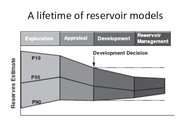
A lifetime of reservoir models
A lifetime of reservoir models
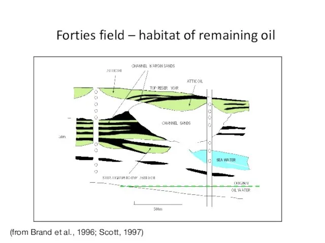
Forties field – habitat of remaining oil
(from Brand et al., 1996;
Forties field – habitat of remaining oil
(from Brand et al., 1996;
Monetary value of an asset
Recoverable resources (i.e. reserves)
Rate of production
Cost of
Monetary value of an asset
Recoverable resources (i.e. reserves)
Rate of production
Cost of
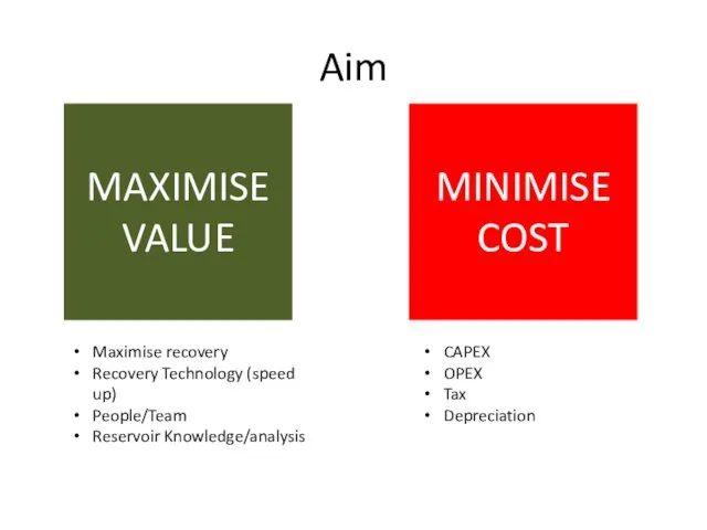
Aim
MAXIMISE
VALUE
MINIMISE
COST
Maximise recovery
Recovery Technology (speed up)
People/Team
Reservoir Knowledge/analysis
CAPEX
OPEX
Tax
Depreciation
Aim
MAXIMISE
VALUE
MINIMISE
COST
Maximise recovery
Recovery Technology (speed up)
People/Team
Reservoir Knowledge/analysis
CAPEX
OPEX
Tax
Depreciation

RECOVERY
Maximise value through…
RECOVERY
Maximise value through…
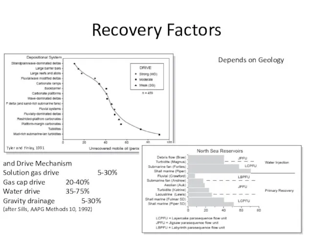
Recovery Factors
Tyler and Finlay, 1991
Depends on Geology
and Drive Mechanism
Solution gas drive
Recovery Factors
Tyler and Finlay, 1991
Depends on Geology
and Drive Mechanism
Solution gas drive
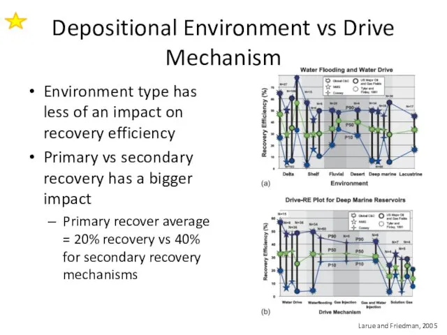
Depositional Environment vs Drive Mechanism
Environment type has less of an impact
Depositional Environment vs Drive Mechanism
Environment type has less of an impact
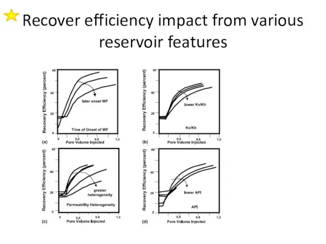
Recover efficiency impact from various reservoir features
Recover efficiency impact from various reservoir features

Does connectivity influence recovery?
Does connectivity influence recovery?
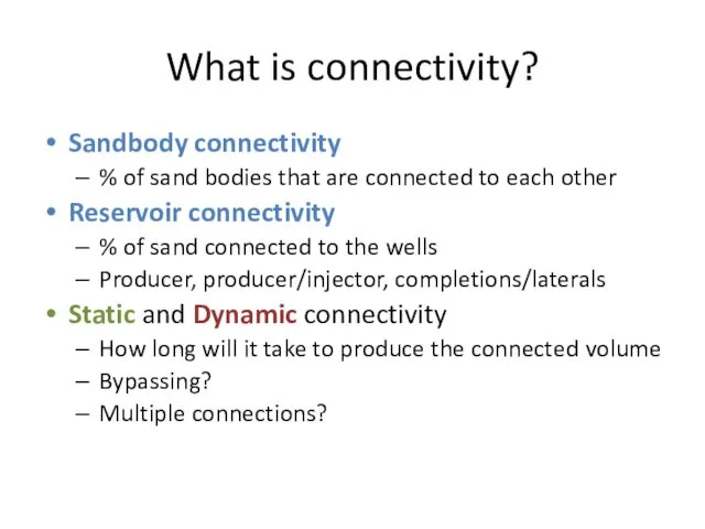
What is connectivity?
Sandbody connectivity
% of sand bodies that are connected
What is connectivity?
Sandbody connectivity
% of sand bodies that are connected
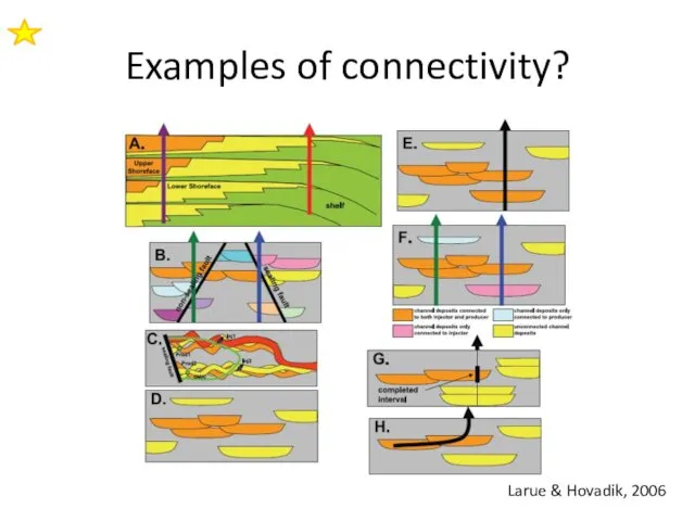
Examples of connectivity?
Larue & Hovadik, 2006
Examples of connectivity?
Larue & Hovadik, 2006
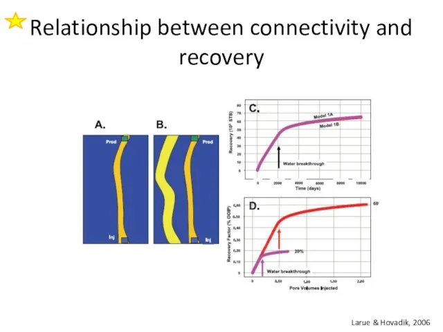
Relationship between connectivity and recovery
Larue & Hovadik, 2006
Relationship between connectivity and recovery
Larue & Hovadik, 2006
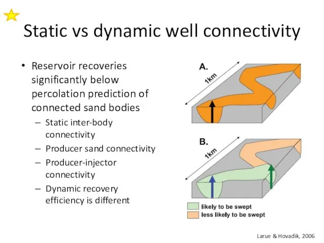
Static vs dynamic well connectivity
Reservoir recoveries significantly below percolation prediction of
Static vs dynamic well connectivity
Reservoir recoveries significantly below percolation prediction of

2D Connectivity
Hovadik & Larue, 2010
2D Connectivity
Hovadik & Larue, 2010
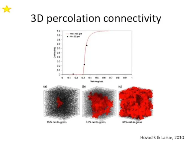
3D percolation connectivity
Hovadik & Larue, 2010
3D percolation connectivity
Hovadik & Larue, 2010
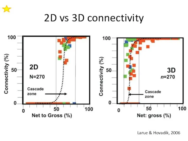
2D vs 3D connectivity
Larue & Hovadik, 2006
2D vs 3D connectivity
Larue & Hovadik, 2006
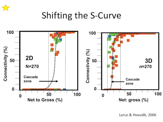
Shifting the S-Curve
Larue & Hovadik, 2006
Shifting the S-Curve
Larue & Hovadik, 2006
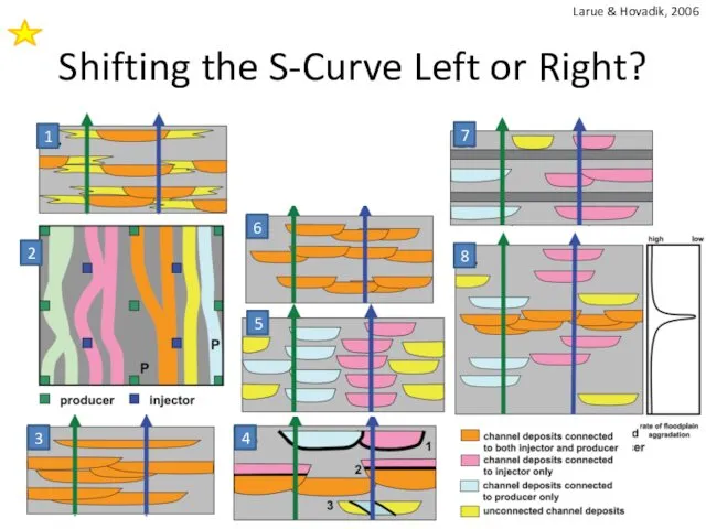
Shifting the S-Curve Left or Right?
1
2
3
6
7
8
5
4
Larue & Hovadik, 2006
Shifting the S-Curve Left or Right?
1
2
3
6
7
8
5
4
Larue & Hovadik, 2006
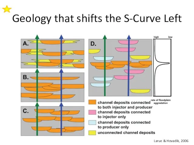
Geology that shifts the S-Curve Left
Larue & Hovadik, 2006
Geology that shifts the S-Curve Left
Larue & Hovadik, 2006
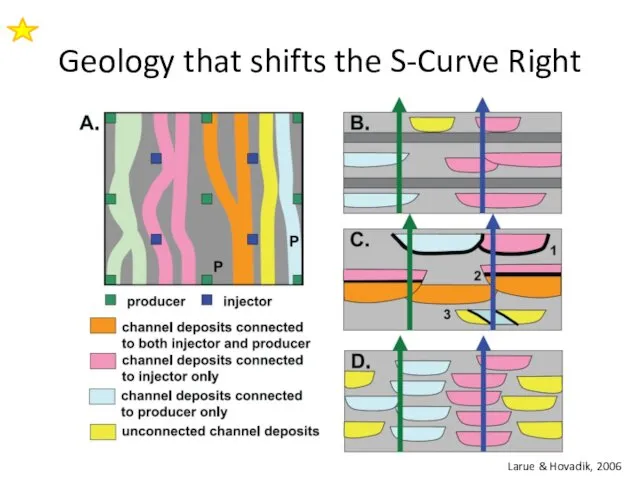
Geology that shifts the S-Curve Right
Larue & Hovadik, 2006
Geology that shifts the S-Curve Right
Larue & Hovadik, 2006
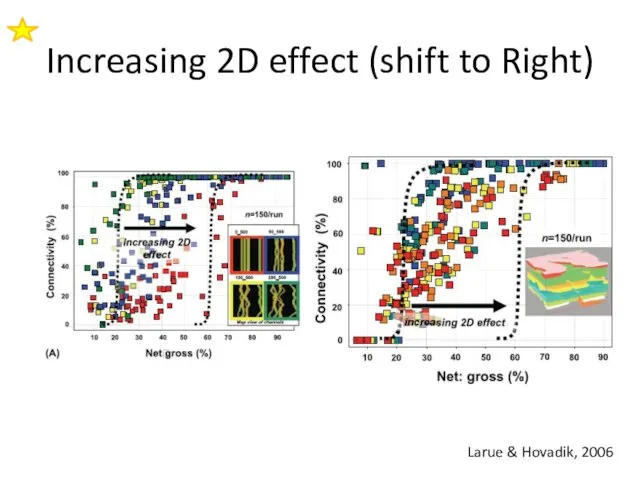
Increasing 2D effect (shift to Right)
Larue & Hovadik, 2006
Increasing 2D effect (shift to Right)
Larue & Hovadik, 2006
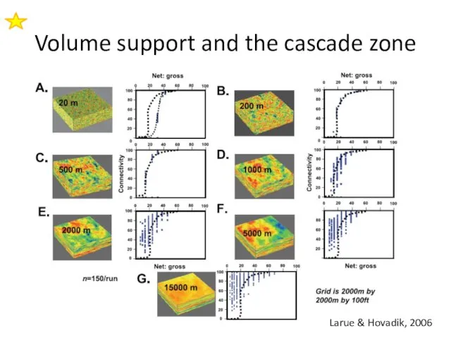
Volume support and the cascade zone
Larue & Hovadik, 2006
Volume support and the cascade zone
Larue & Hovadik, 2006
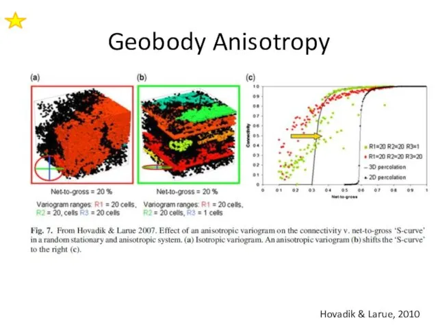
Geobody Anisotropy
Hovadik & Larue, 2010
Geobody Anisotropy
Hovadik & Larue, 2010
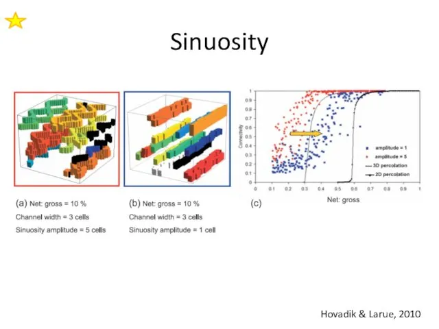
Sinuosity
Hovadik & Larue, 2010
Sinuosity
Hovadik & Larue, 2010
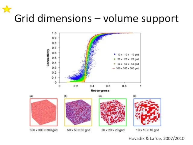
Grid dimensions – volume support
Hovadik & Larue, 2007/2010
Grid dimensions – volume support
Hovadik & Larue, 2007/2010
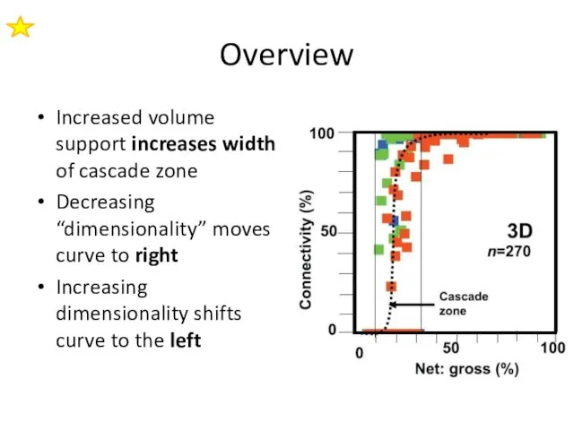
Overview
Increased volume support increases width of cascade zone
Decreasing “dimensionality” moves curve
Overview
Increased volume support increases width of cascade zone
Decreasing “dimensionality” moves curve
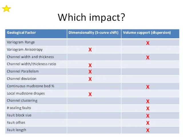
Which impact?
X
X
X
X
X
X
X
X
X
X
X
X
X
Which impact?
X
X
X
X
X
X
X
X
X
X
X
X
X
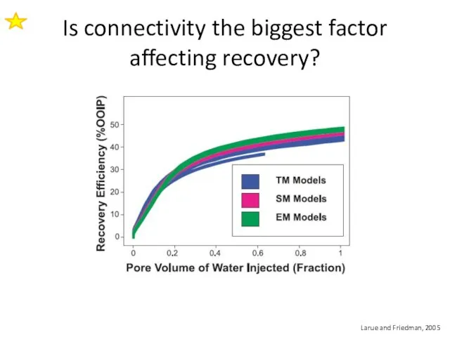
Is connectivity the biggest factor affecting recovery?
Larue and Friedman, 2005
Is connectivity the biggest factor affecting recovery?
Larue and Friedman, 2005
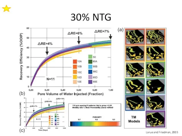
30% NTG
Larue and Friedman, 2005
30% NTG
Larue and Friedman, 2005
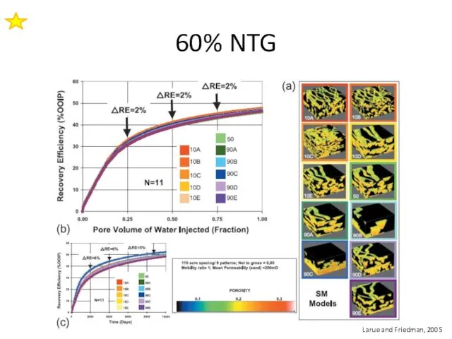
60% NTG
Larue and Friedman, 2005
60% NTG
Larue and Friedman, 2005
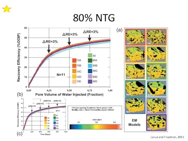
80% NTG
Larue and Friedman, 2005
80% NTG
Larue and Friedman, 2005
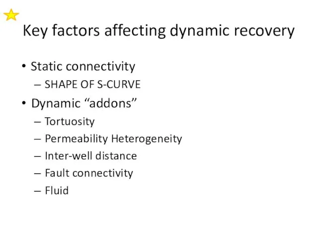
Key factors affecting dynamic recovery
Static connectivity
SHAPE OF S-CURVE
Dynamic “addons”
Tortuosity
Permeability Heterogeneity
Inter-well distance
Fault
Key factors affecting dynamic recovery
Static connectivity
SHAPE OF S-CURVE
Dynamic “addons”
Tortuosity
Permeability Heterogeneity
Inter-well distance
Fault
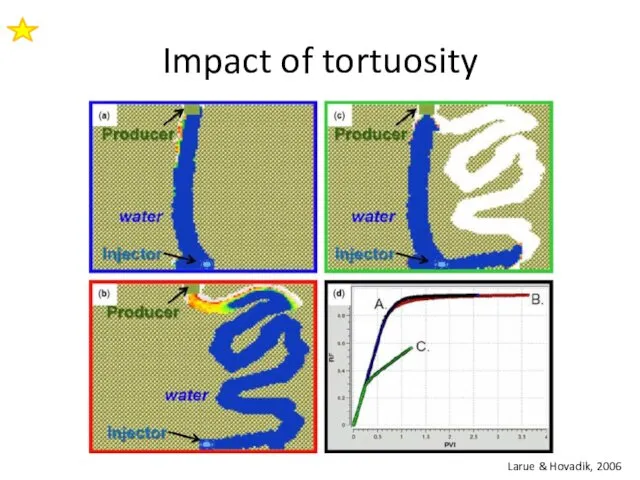
Impact of tortuosity
Larue & Hovadik, 2006
Impact of tortuosity
Larue & Hovadik, 2006
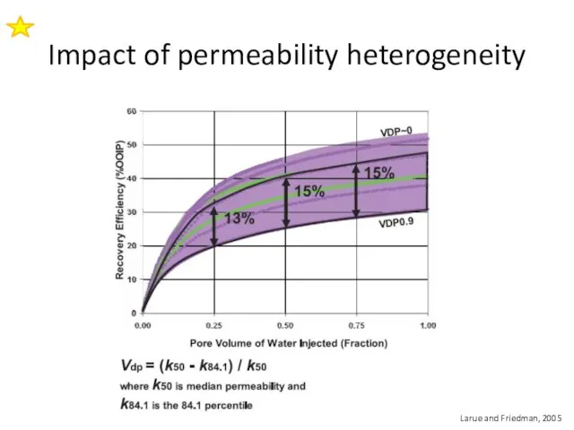
Impact of permeability heterogeneity
Larue and Friedman, 2005
Impact of permeability heterogeneity
Larue and Friedman, 2005
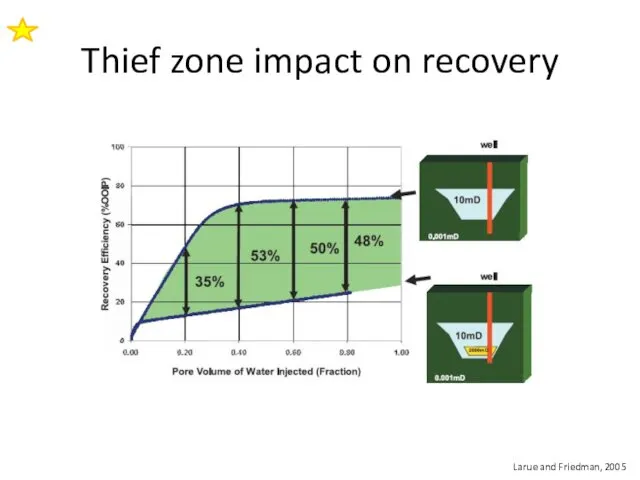
Thief zone impact on recovery
Larue and Friedman, 2005
Thief zone impact on recovery
Larue and Friedman, 2005
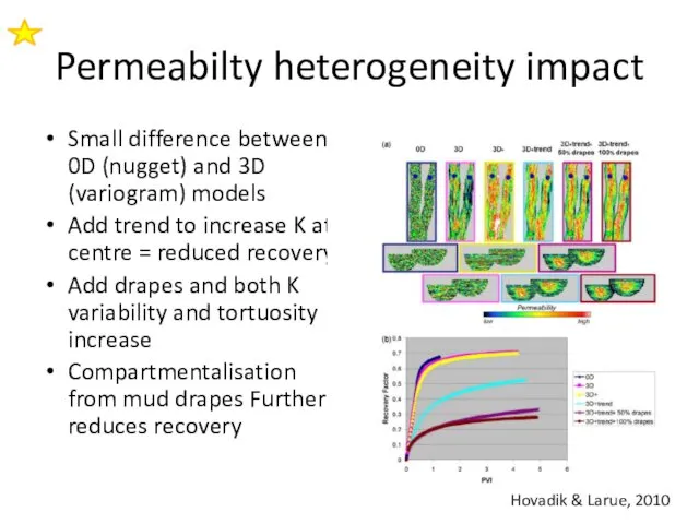
Permeabilty heterogeneity impact
Small difference between 0D (nugget) and 3D (variogram) models
Add
Permeabilty heterogeneity impact
Small difference between 0D (nugget) and 3D (variogram) models
Add
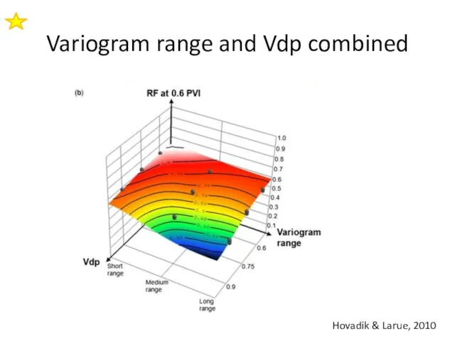
Variogram range and Vdp combined
Hovadik & Larue, 2010
Variogram range and Vdp combined
Hovadik & Larue, 2010
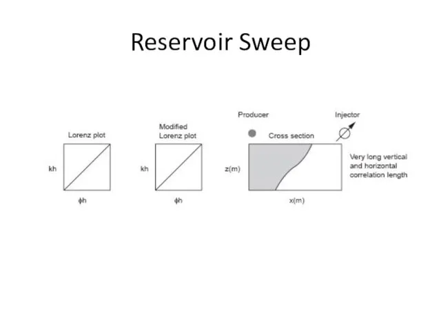
Reservoir Sweep
Reservoir Sweep
Reservoir Sweep
Reservoir Sweep
Reservoir Sweep
Reservoir Sweep
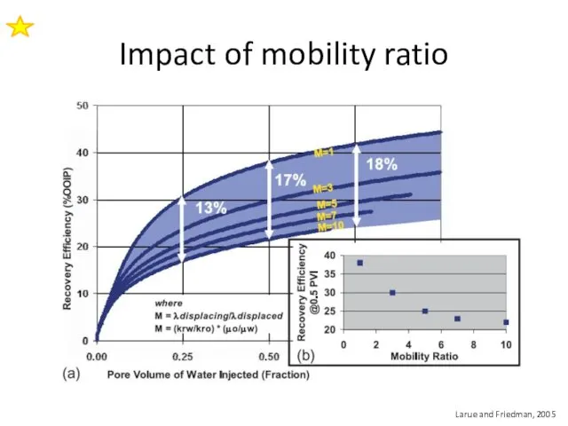
Impact of mobility ratio
Larue and Friedman, 2005
Impact of mobility ratio
Larue and Friedman, 2005
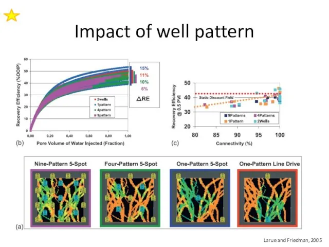
Impact of well pattern
Larue and Friedman, 2005
Impact of well pattern
Larue and Friedman, 2005
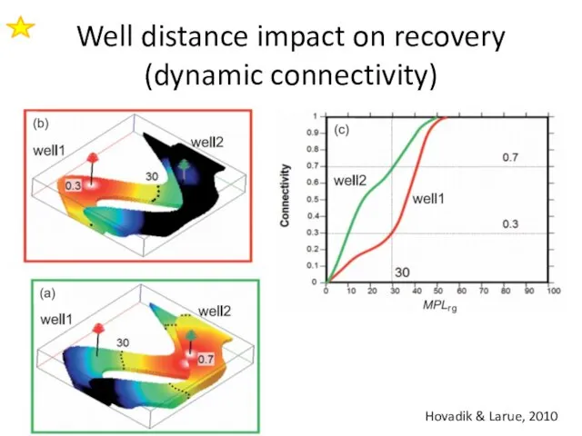
Well distance impact on recovery (dynamic connectivity)
Hovadik & Larue, 2010
Well distance impact on recovery (dynamic connectivity)
Hovadik & Larue, 2010
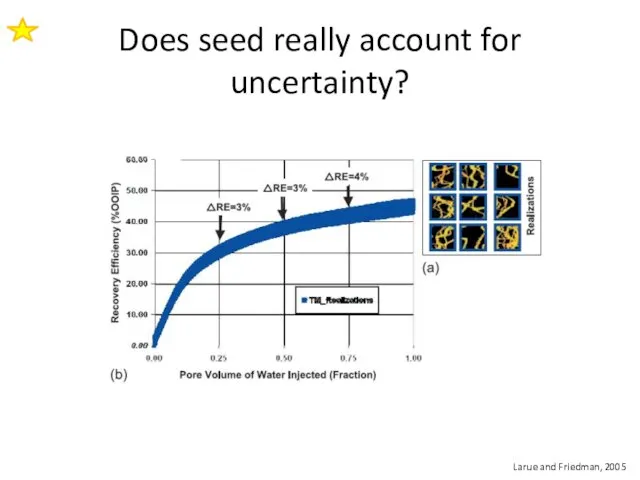
Does seed really account for uncertainty?
Larue and Friedman, 2005
Does seed really account for uncertainty?
Larue and Friedman, 2005
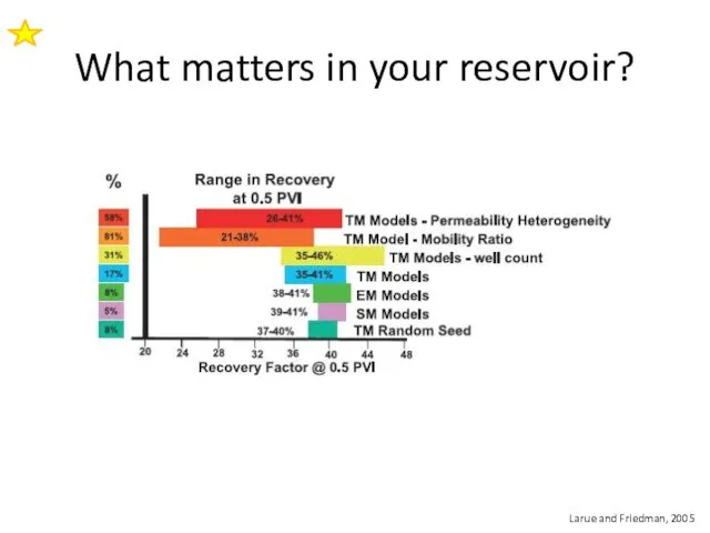
What matters in your reservoir?
Larue and Friedman, 2005
What matters in your reservoir?
Larue and Friedman, 2005

Extreme edge cases: High NTG + Low Connectivity
Manzocchi et al, 2007
Extreme edge cases: High NTG + Low Connectivity
Manzocchi et al, 2007
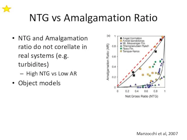
NTG vs Amalgamation Ratio
NTG and Amalgamation ratio do not corellate in
NTG vs Amalgamation Ratio
NTG and Amalgamation ratio do not corellate in
Object Based Modelling
Convergence Problem
Illustration of Sequential
Object Based Algorithm (Srivastava 1994)
As Number
Object Based Modelling
Convergence Problem
Illustration of Sequential
Object Based Algorithm (Srivastava 1994)
As Number
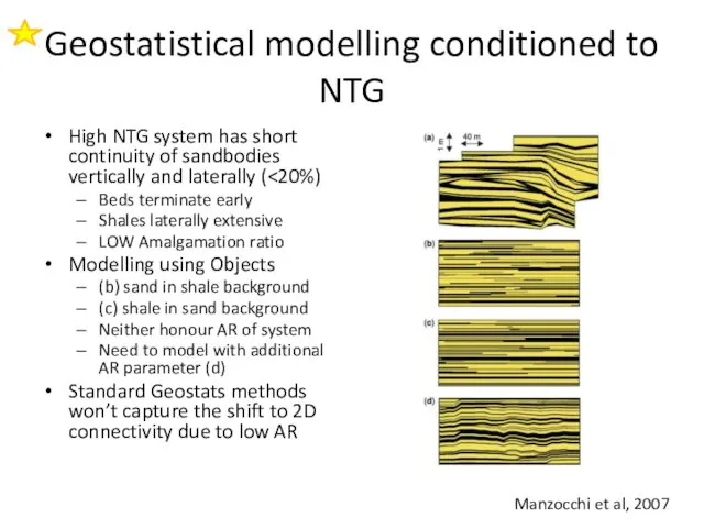
Geostatistical modelling conditioned to NTG
High NTG system has short continuity of
Geostatistical modelling conditioned to NTG
High NTG system has short continuity of
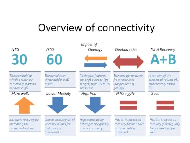
Overview of connectivity
30%
60%
A+B
NTG
NTG
Geobody size
Total Recovery
Impact of Geology
More wells
Lower Mobility
High Vdp
NTG >35%
Seed
Overview of connectivity
30%
60%
A+B
NTG
NTG
Geobody size
Total Recovery
Impact of Geology
More wells
Lower Mobility
High Vdp
NTG >35%
Seed

IMPROVED RECOVERY
Maximise value through…
IMPROVED RECOVERY
Maximise value through…

Recovery Factors
Tyler and Finlay, 1991
Depends on Geology
and Drive Mechanism
Solution gas drive
Recovery Factors
Tyler and Finlay, 1991
Depends on Geology
and Drive Mechanism
Solution gas drive
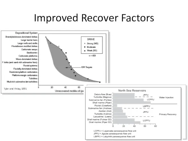
Improved Recover Factors
Tyler and Finlay, 1991
Improved Recover Factors
Tyler and Finlay, 1991
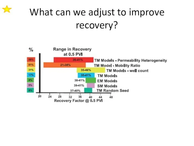
What can we adjust to improve recovery?
What can we adjust to improve recovery?
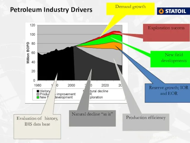
Evaluation of history, IHS data base
Natural decline “as is”
Production efficiency
Reserve growth;
Evaluation of history, IHS data base
Natural decline “as is”
Production efficiency
Reserve growth;
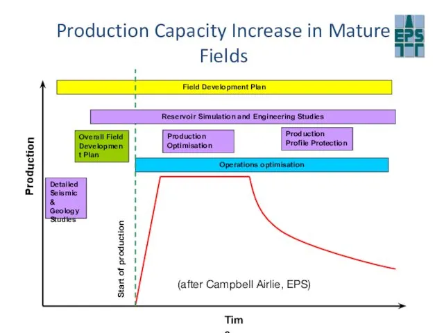
Production Capacity Increase in Mature Fields
Time
Production
Overall Field Development Plan
Detailed Seismic &
Production Capacity Increase in Mature Fields
Time
Production
Overall Field Development Plan
Detailed Seismic &
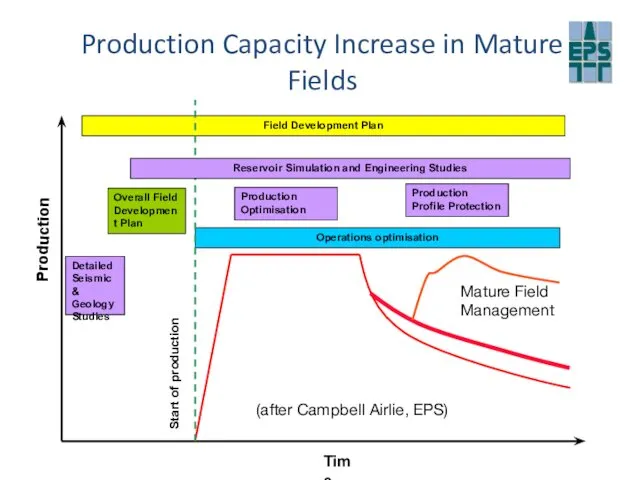
Production Capacity Increase in Mature Fields
Time
Production
Overall Field Development Plan
Detailed Seismic &
Production Capacity Increase in Mature Fields
Time
Production
Overall Field Development Plan
Detailed Seismic &

INFILL DRILLING
Example of….
INFILL DRILLING
Example of….
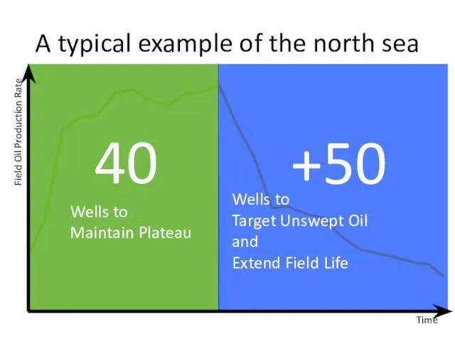
Time
Field Oil Production Rate
A typical example of the north sea
Time
Field Oil Production Rate
A typical example of the north sea
RM Example 1
Strategy for Statfjord
Aadland et al., 1994
High well activity
Horizontal wells
Reservoir
RM Example 1
Strategy for Statfjord
Aadland et al., 1994
High well activity
Horizontal wells
Reservoir
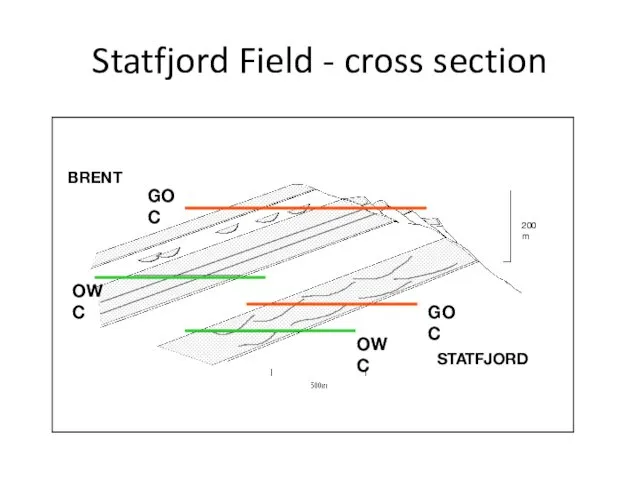
Statfjord Field - cross section
GOC
OWC
GOC
OWC
BRENT
STATFJORD
200m
Statfjord Field - cross section
GOC
OWC
GOC
OWC
BRENT
STATFJORD
200m
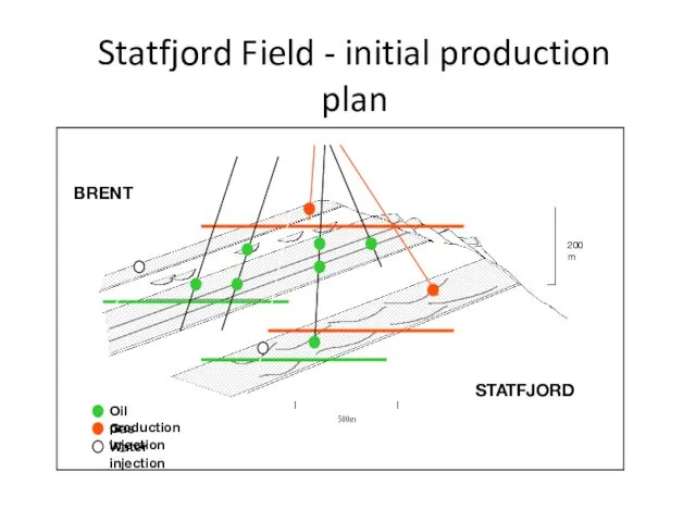
Statfjord Field - initial production plan
BRENT
STATFJORD
200m
Water injection
Gas injection
Oil production
Statfjord Field - initial production plan
BRENT
STATFJORD
200m
Water injection
Gas injection
Oil production
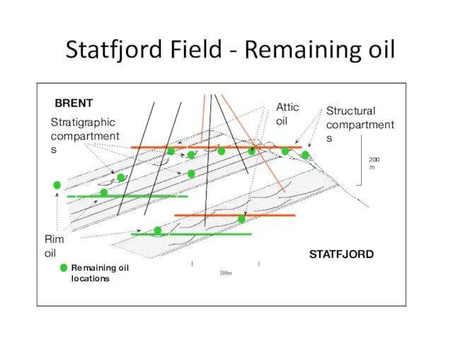
Statfjord Field - Remaining oil
BRENT
STATFJORD
200m
Remaining oil locations
Rim oil
Attic oil
Structural compartments
Stratigraphic
compartments
Statfjord Field - Remaining oil
BRENT
STATFJORD
200m
Remaining oil locations
Rim oil
Attic oil
Structural compartments
Stratigraphic
compartments
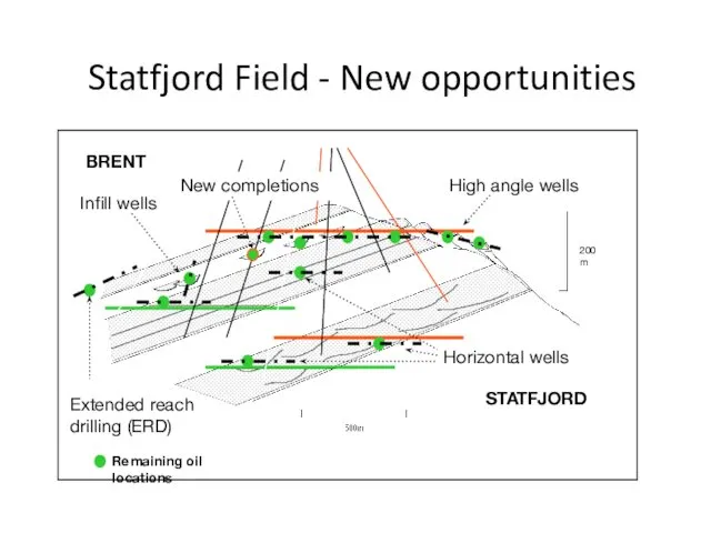
Statfjord Field - New opportunities
BRENT
STATFJORD
200m
Remaining oil locations
New completions
Horizontal wells
High angle wells
Extended
Statfjord Field - New opportunities
BRENT
STATFJORD
200m
Remaining oil locations
New completions
Horizontal wells
High angle wells
Extended
Example: Yibal Field, Oman
Strategy for Yibal Field, Oman
Horizontal wells
Bypassed oil in
Example: Yibal Field, Oman
Strategy for Yibal Field, Oman
Horizontal wells
Bypassed oil in
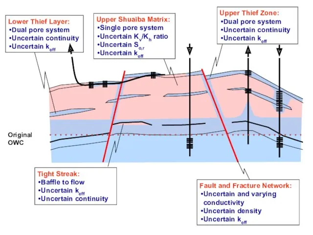
Modelling Characteristics and Sensitivities
Original OWC
Upper Shuaiba Matrix:
Single pore system
Uncertain Kv/Kh ratio
Uncertain
Modelling Characteristics and Sensitivities
Original OWC
Upper Shuaiba Matrix:
Single pore system
Uncertain Kv/Kh ratio
Uncertain

Yibal Field Development History
Depletion and “phase” injection
Aquifer injection
Onset of horizontal drilling
High
Yibal Field Development History
Depletion and “phase” injection
Aquifer injection
Onset of horizontal drilling
High

YIBAL FIELD: Water - Oil Rate vs RF
Phase
Aquifer Injection
Horizontals
01/81
01/88
01/94
09/98
YIBAL FIELD: Water - Oil Rate vs RF
Phase
Aquifer Injection
Horizontals
01/81
01/88
01/94
09/98
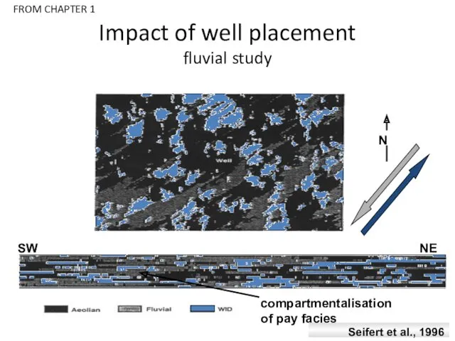
Seifert et al., 1996
Impact of well placement
fluvial study
SW
NE
compartmentalisation
of pay facies
FROM CHAPTER
Seifert et al., 1996
Impact of well placement
fluvial study
SW
NE
compartmentalisation
of pay facies
FROM CHAPTER
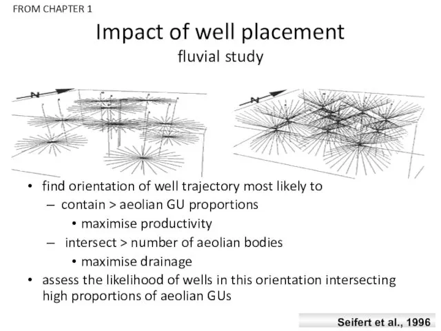
Seifert et al., 1996
Impact of well placement
fluvial study
find orientation of well
Seifert et al., 1996
Impact of well placement
fluvial study
find orientation of well
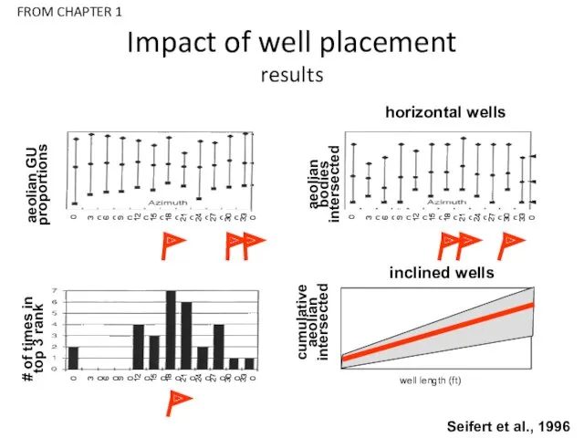
Seifert et al., 1996
Impact of well placement
results
aeolian bodies
intersected
aeolian GU
proportions
horizontal wells
#
Seifert et al., 1996
Impact of well placement
results
aeolian bodies
intersected
aeolian GU
proportions
horizontal wells
#
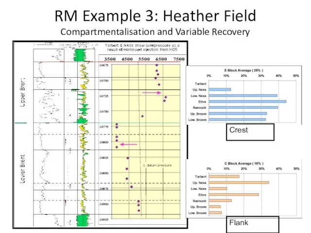
RM Example 3: Heather Field
Compartmentalisation and Variable Recovery
Crest
Flank
RM Example 3: Heather Field
Compartmentalisation and Variable Recovery
Crest
Flank
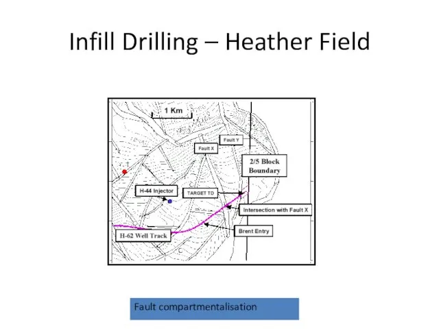
Infill Drilling – Heather Field
Fault compartmentalisation
Infill Drilling – Heather Field
Fault compartmentalisation

FRACCING
Example of….
FRACCING
Example of….
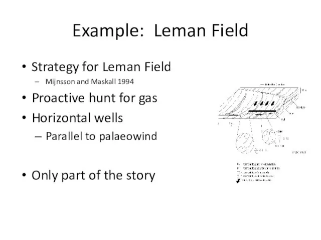
Example: Leman Field
Strategy for Leman Field
Mijnsson and Maskall 1994
Proactive hunt for
Example: Leman Field
Strategy for Leman Field
Mijnsson and Maskall 1994
Proactive hunt for
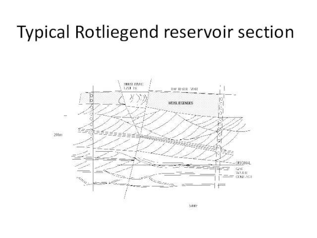
Typical Rotliegend reservoir section
Typical Rotliegend reservoir section
Typical Rotliegend reservoir section
Bypassed gas
Stratigraphic/structurally bypassed gas
Typical Rotliegend reservoir section
Bypassed gas
Stratigraphic/structurally bypassed gas
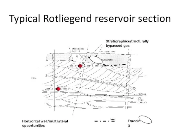
Typical Rotliegend reservoir section
Horizontal well/multilateral opportunities
Stratigraphic/structurally bypassed gas
Fraccing
Typical Rotliegend reservoir section
Horizontal well/multilateral opportunities
Stratigraphic/structurally bypassed gas
Fraccing

EOR (WAG)
Example of….
EOR (WAG)
Example of….
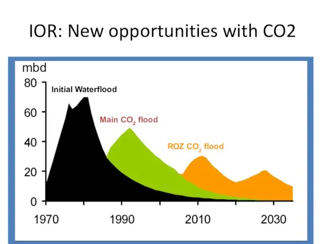
IOR: New opportunities with CO2
Initial Waterflood
Main CO2 flood
ROZ CO2 flood
mbd
IOR: New opportunities with CO2
Initial Waterflood
Main CO2 flood
ROZ CO2 flood
mbd
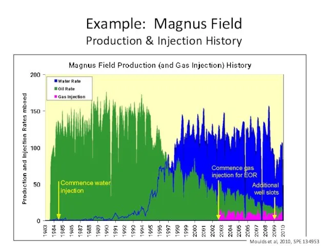
Example: Magnus Field
Production & Injection History
Commence water injection
Moulds et al, 2010,
Example: Magnus Field
Production & Injection History
Commence water injection
Moulds et al, 2010,
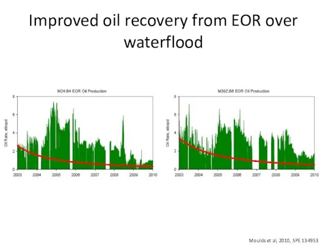
Improved oil recovery from EOR over waterflood
Moulds et al, 2010, SPE
Improved oil recovery from EOR over waterflood
Moulds et al, 2010, SPE
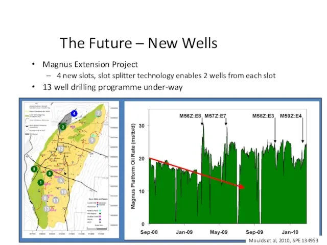
The Future – New Wells
Magnus Extension Project
4 new slots, slot splitter
The Future – New Wells
Magnus Extension Project
4 new slots, slot splitter
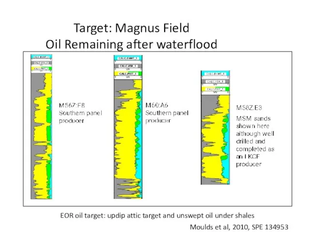
Target: Magnus Field
Oil Remaining after waterflood
EOR oil target: updip
Target: Magnus Field
Oil Remaining after waterflood
EOR oil target: updip

PEOPLE/TEAMS
Maximise value through…
PEOPLE/TEAMS
Maximise value through…
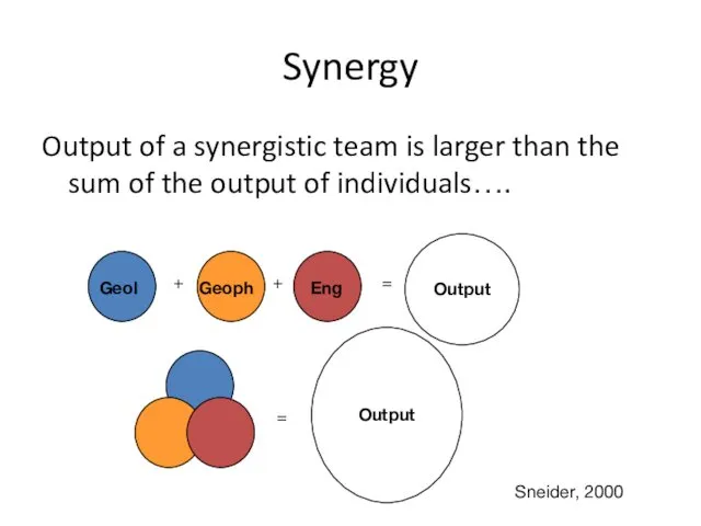
Synergy
Output of a synergistic team is larger than the sum of
Synergy
Output of a synergistic team is larger than the sum of

Synergy
Is not:
Geoengineering
Any thing about multi-discipline work
Anything to do with Energy
Synergy
Sum of
Synergy
Is not:
Geoengineering
Any thing about multi-discipline work
Anything to do with Energy
Synergy
Sum of
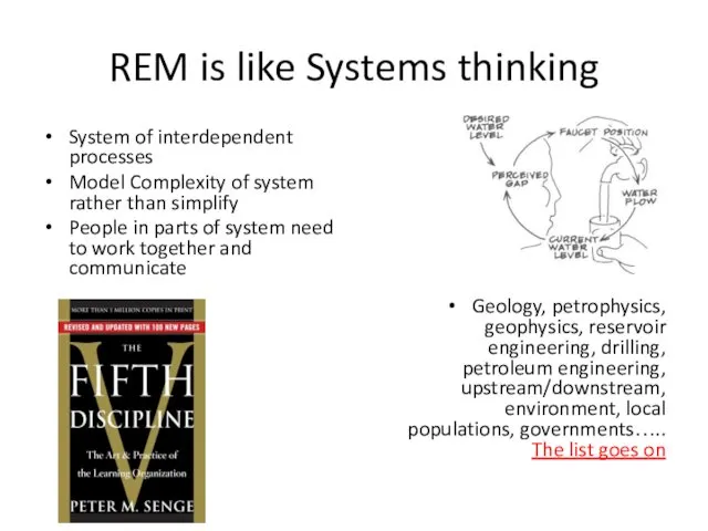
REM is like Systems thinking
System of interdependent processes
Model Complexity of system
REM is like Systems thinking
System of interdependent processes
Model Complexity of system
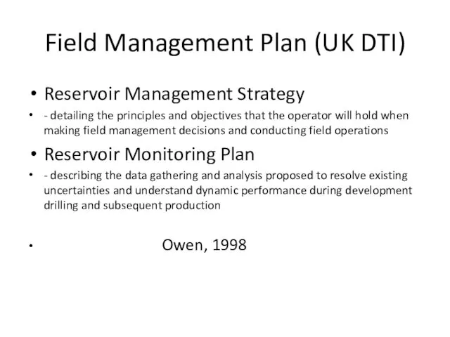
Field Management Plan (UK DTI)
Reservoir Management Strategy
- detailing the principles and
Field Management Plan (UK DTI)
Reservoir Management Strategy
- detailing the principles and
RM Strategy
Developing
Implementing
Monitoring
Evaluating
DIME - Satter and Thakur, 1994
RM Strategy
Developing
Implementing
Monitoring
Evaluating
DIME - Satter and Thakur, 1994

WATER MANAGEMENT
Increase costs through…
WATER MANAGEMENT
Increase costs through…
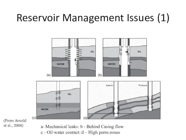
Reservoir Management Issues (1)
a- Mechanical leaks: b - Behind Casing flow
Reservoir Management Issues (1)
a- Mechanical leaks: b - Behind Casing flow
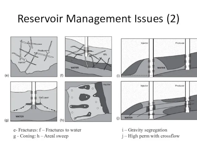
Reservoir Management Issues (2)
e- Fractures: f – Fractures to water
g
Reservoir Management Issues (2)
e- Fractures: f – Fractures to water
g

WATER SHUTOFF
Example of….
WATER SHUTOFF
Example of….
Yibal Field Development History
Depletion and “phase” injection
Aquifer injection
Onset of horizontal drilling
High
Yibal Field Development History
Depletion and “phase” injection
Aquifer injection
Onset of horizontal drilling
High
YIBAL FIELD: Water - Oil Rate vs RF
Phase
Aquifer Injection
Horizontals
01/81
01/88
01/94
09/98
YIBAL FIELD: Water - Oil Rate vs RF
Phase
Aquifer Injection
Horizontals
01/81
01/88
01/94
09/98
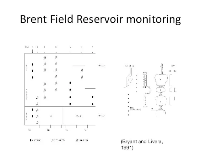
Brent Field Reservoir monitoring
(Bryant and Livera, 1991)
Brent Field Reservoir monitoring
(Bryant and Livera, 1991)
Brent Field Reservoir monitoring
(Bryant and Livera, 1991)
1. Initial Conditions
Ness Formation
Brent Field Reservoir monitoring
(Bryant and Livera, 1991)
1. Initial Conditions
Ness Formation
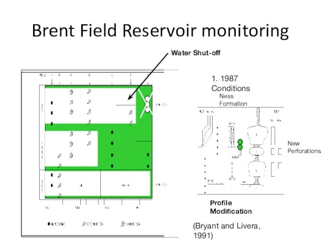
Brent Field Reservoir monitoring
(Bryant and Livera, 1991)
1. 1987 Conditions
Ness Formation
New Perforations
Profile
Brent Field Reservoir monitoring
(Bryant and Livera, 1991)
1. 1987 Conditions
Ness Formation
New Perforations
Profile

SCALE MANAGEMENT
Increase costs through…
SCALE MANAGEMENT
Increase costs through…
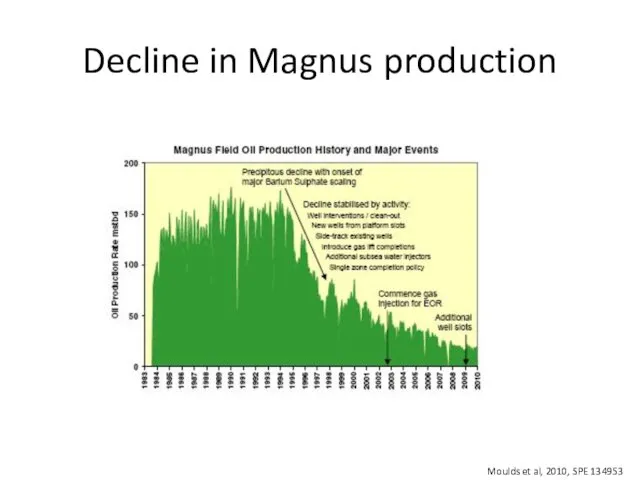
Decline in Magnus production
Moulds et al, 2010, SPE 134953
Decline in Magnus production
Moulds et al, 2010, SPE 134953
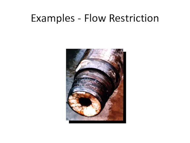
Examples - Flow Restriction
Examples - Flow Restriction
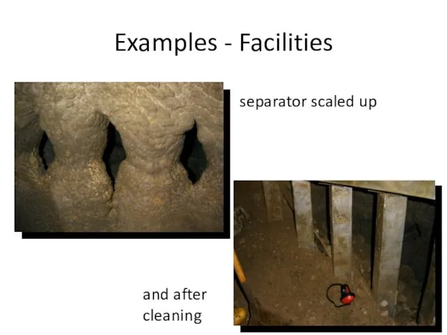
Examples - Facilities
separator scaled up
and after
cleaning
Examples - Facilities
separator scaled up
and after
cleaning
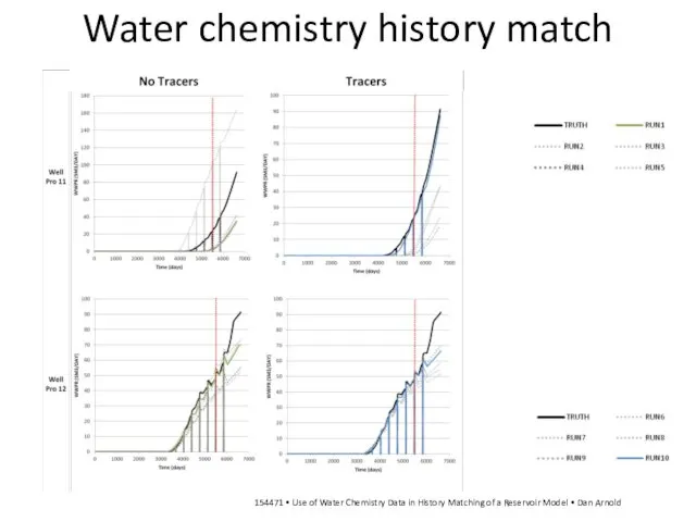
Water chemistry history match
154471 • Use of Water Chemistry Data in
Water chemistry history match
154471 • Use of Water Chemistry Data in
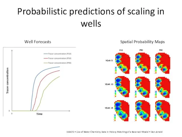
Probabilistic predictions of scaling in wells
154471 • Use of Water Chemistry
Probabilistic predictions of scaling in wells
154471 • Use of Water Chemistry
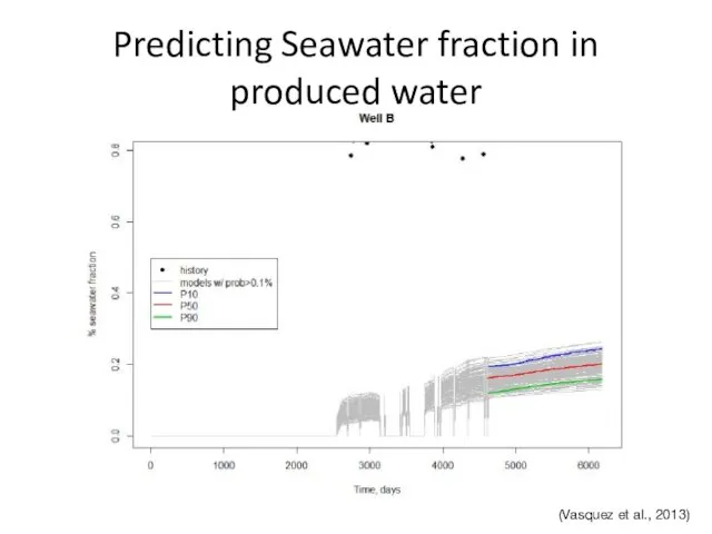
Predicting Seawater fraction in produced water
(Vasquez et al., 2013)
Predicting Seawater fraction in produced water
(Vasquez et al., 2013)

Probability maps of seawater fraction
P10
P50
P90
Probability maps of seawater fraction
P10
P50
P90
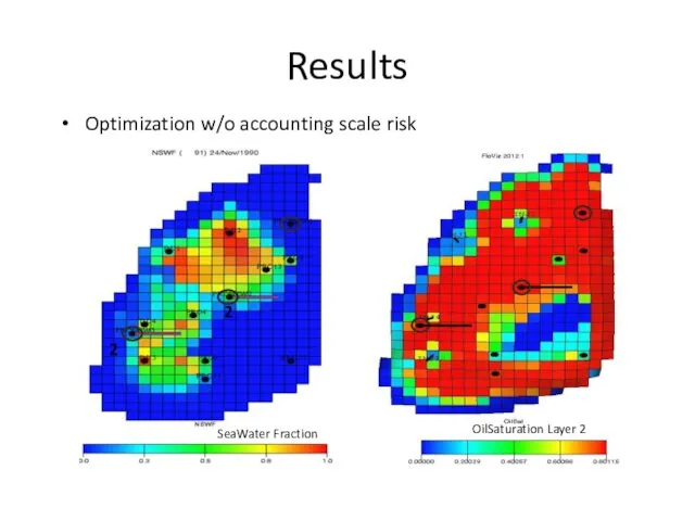
Results
Optimization w/o accounting scale risk
Results
Optimization w/o accounting scale risk
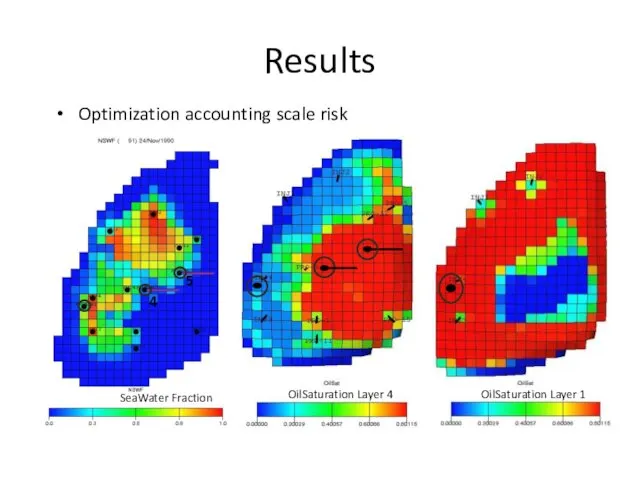
Results
Optimization accounting scale risk
SeaWater Fraction
OilSaturation Layer 4
OilSaturation Layer 1
Results
Optimization accounting scale risk
SeaWater Fraction
OilSaturation Layer 4
OilSaturation Layer 1
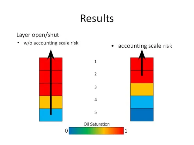
Results
Layer open/shut
w/o accounting scale risk
accounting scale risk
0
1
Results
Layer open/shut
w/o accounting scale risk
accounting scale risk
0
1

Impact in the value through…
VALUE OF YOUR OIL
Impact in the value through…
VALUE OF YOUR OIL
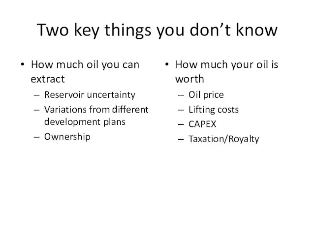
Two key things you don’t know
How much oil you can extract
Reservoir
Two key things you don’t know
How much oil you can extract
Reservoir
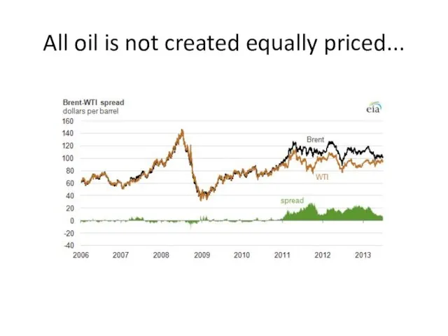
All oil is not created equally priced...
All oil is not created equally priced...

Time value of money
where
DPV is the discounted present value of the future
Time value of money
where
DPV is the discounted present value of the future
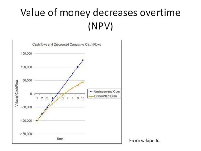
Value of money decreases overtime (NPV)
From wikipedia
Value of money decreases overtime (NPV)
From wikipedia
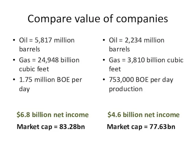
Compare value of companies
Oil = 5,817 million barrels
Gas = 24,948 billion
Compare value of companies
Oil = 5,817 million barrels
Gas = 24,948 billion
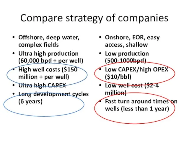
Compare strategy of companies
Offshore, deep water, complex fields
Ultra high production (60,000
Compare strategy of companies
Offshore, deep water, complex fields
Ultra high production (60,000
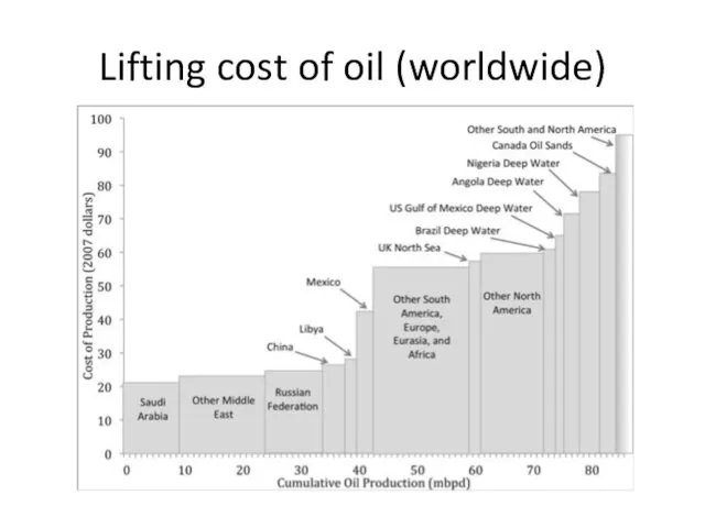
Lifting cost of oil (worldwide)
Lifting cost of oil (worldwide)
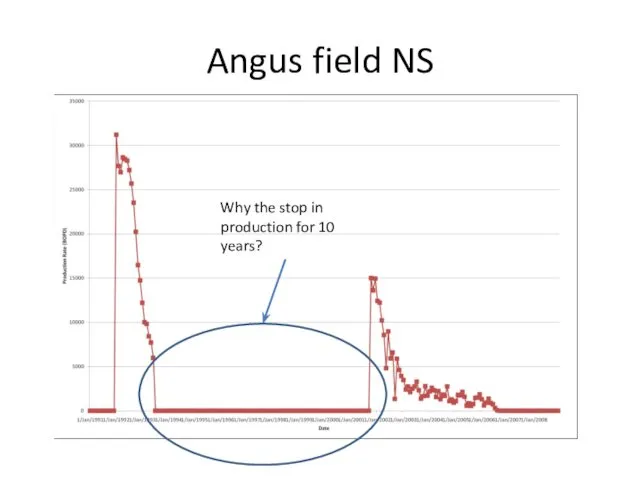
Angus field NS
Why the stop in production for 10 years?
Angus field NS
Why the stop in production for 10 years?
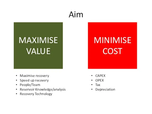
Aim
MAXIMISE
VALUE
MINIMISE
COST
Maximise recovery
Speed up recovery
People/Team
Reservoir Knowledge/analysis
Recovery Technology
CAPEX
OPEX
Tax
Depreciation
Aim
MAXIMISE
VALUE
MINIMISE
COST
Maximise recovery
Speed up recovery
People/Team
Reservoir Knowledge/analysis
Recovery Technology
CAPEX
OPEX
Tax
Depreciation
Aim
MAXIMISE
VALUE
MINIMISE
COST
Maximise recovery
Speed up recovery
People/Team
Reservoir Knowledge/analysis
Recovery Technology
CAPEX
OPEX
Tax
Depreciation
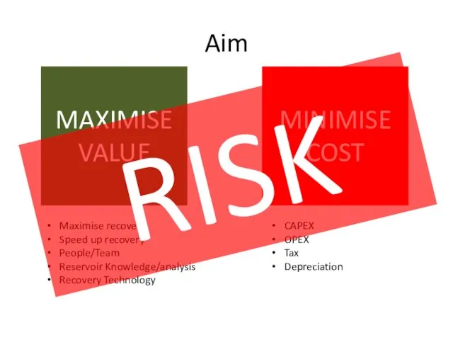
RISK
Aim
MAXIMISE
VALUE
MINIMISE
COST
Maximise recovery
Speed up recovery
People/Team
Reservoir Knowledge/analysis
Recovery Technology
CAPEX
OPEX
Tax
Depreciation
RISK
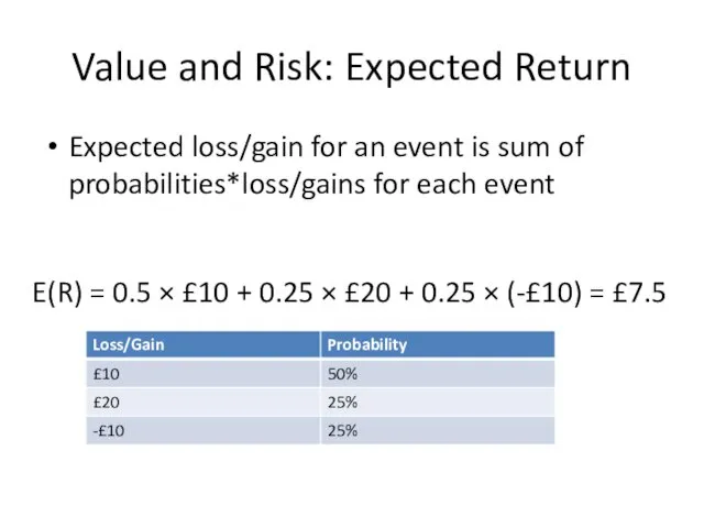
Value and Risk: Expected Return
Expected loss/gain for an event is sum
Value and Risk: Expected Return
Expected loss/gain for an event is sum
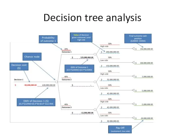
Decision tree analysis
Decision tree analysis
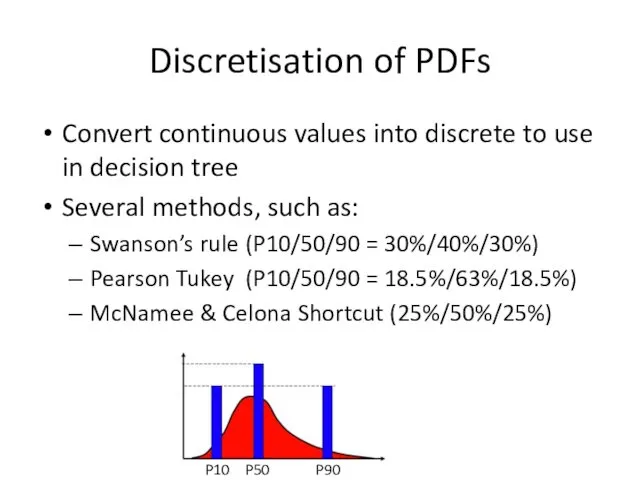
Discretisation of PDFs
Convert continuous values into discrete to use in decision
Discretisation of PDFs
Convert continuous values into discrete to use in decision

RESERVOIR DEVELOPMENT OPTIMISATION
Maximise value through…
RESERVOIR DEVELOPMENT OPTIMISATION
Maximise value through…

What do we mean by optimisation
Process of improving something
to find the
What do we mean by optimisation
Process of improving something
to find the
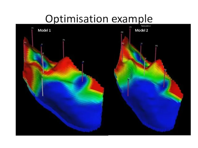
Optimisation example
Model 1
Model 2
Optimisation example
Model 1
Model 2
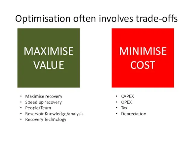
Optimisation often involves trade-offs
MAXIMISE
VALUE
MINIMISE
COST
Maximise recovery
Speed up recovery
People/Team
Reservoir Knowledge/analysis
Recovery Technology
CAPEX
OPEX
Tax
Depreciation
Optimisation often involves trade-offs
MAXIMISE
VALUE
MINIMISE
COST
Maximise recovery
Speed up recovery
People/Team
Reservoir Knowledge/analysis
Recovery Technology
CAPEX
OPEX
Tax
Depreciation

Automated optimisation
A set of algorithms available that can automate the optimisation
Automated optimisation
A set of algorithms available that can automate the optimisation
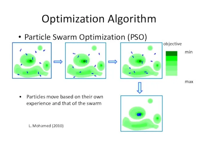
Optimization Algorithm
Particle Swarm Optimization (PSO)
Particles move based on their own experience
Optimization Algorithm
Particle Swarm Optimization (PSO)
Particles move based on their own experience
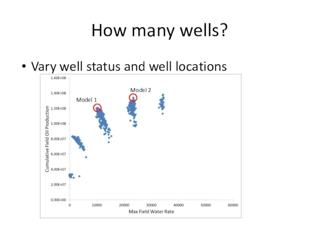
How many wells?
Vary well status and well locations
Model 1
Model 2
How many wells?
Vary well status and well locations
Model 1
Model 2
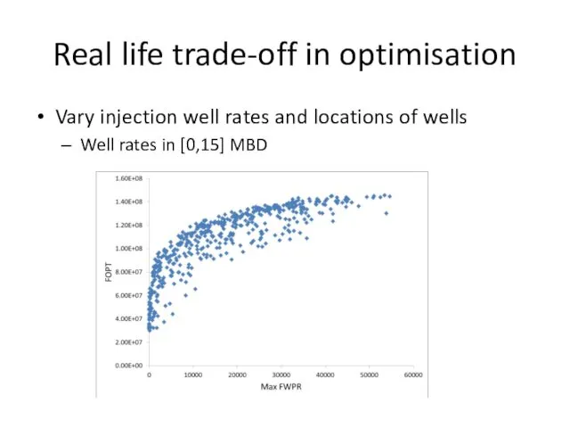
Real life trade-off in optimisation
Vary injection well rates and locations of
Real life trade-off in optimisation
Vary injection well rates and locations of
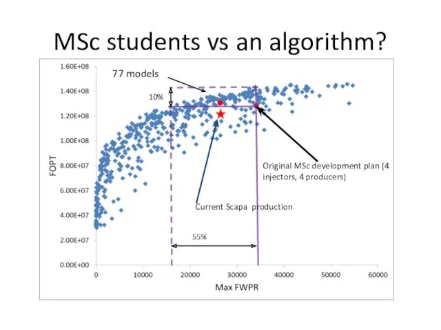
MSc students vs an algorithm?
Original MSc development plan (4 injectors, 4
MSc students vs an algorithm?
Original MSc development plan (4 injectors, 4
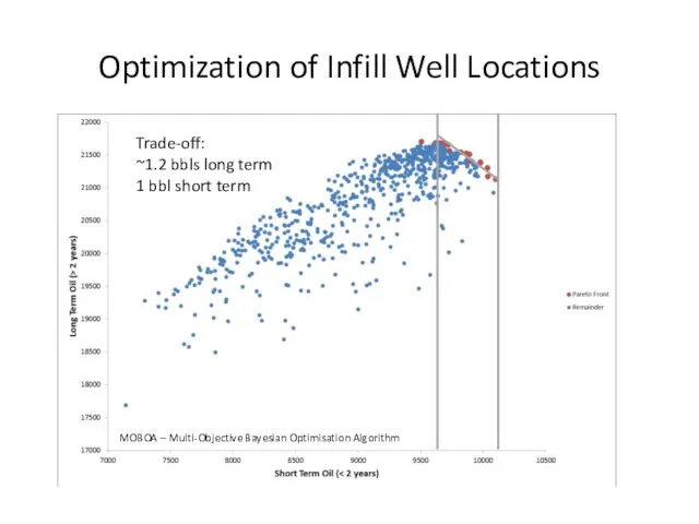
Optimization of Infill Well Locations
Trade-off:
~1.2 bbls long term
1 bbl short
Optimization of Infill Well Locations
Trade-off:
~1.2 bbls long term
1 bbl short

In review
Creating value from of our asset
Ongoing, Life-of-field process
Risk in decisions
In review
Creating value from of our asset
Ongoing, Life-of-field process
Risk in decisions
Summary of strategies
Developing plans
Maximise oil/gas prod. – field rehabilitation
Implementing
SOA facilities and
Summary of strategies
Developing plans
Maximise oil/gas prod. – field rehabilitation
Implementing
SOA facilities and
RM Strategy
Evaluating
Developing
Implmenting
Monitoring
EDIM - as in Edim-bourg……….
RM Strategy
Evaluating
Developing
Implmenting
Monitoring
EDIM - as in Edim-bourg……….

Reservoir Management - key points
Integration
Synergy
Persistence
Proactive
Reservoir Management - key points
Integration
Synergy
Persistence
Proactive

Optimization Algorithm
Particle Swarm Optimization (PSO)
Particles move based on their own experience
Optimization Algorithm
Particle Swarm Optimization (PSO)
Particles move based on their own experience
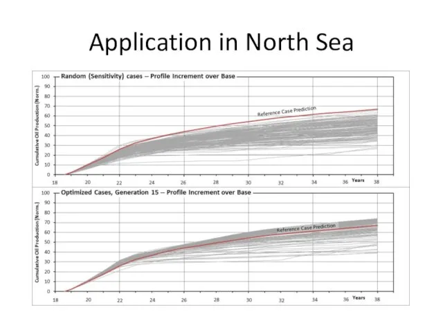
Application in North Sea
Application in North Sea
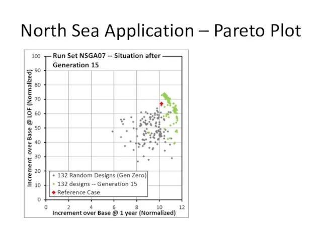
North Sea Application – Pareto Plot
North Sea Application – Pareto Plot

North Sea Application – Pareto Plot
North Sea Application – Pareto Plot
Example: Brent Field
Brent Field Depressurisation
Christiansen and Wilson, 1998, James et al.,
Example: Brent Field
Brent Field Depressurisation
Christiansen and Wilson, 1998, James et al.,
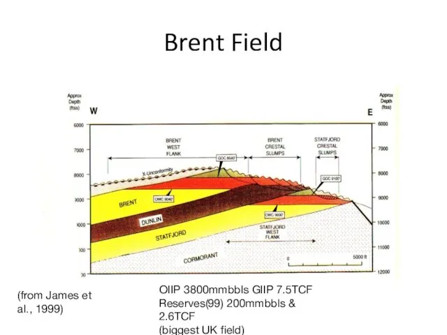
Brent Field
(from James et al., 1999)
OIIP 3800mmbbls GIIP 7.5TCF
Reserves(99) 200mmbbls &
Brent Field
(from James et al., 1999)
OIIP 3800mmbbls GIIP 7.5TCF
Reserves(99) 200mmbbls &
 Землетрясения. Шкала магнитуд
 Соль-Илецк. Ключевая информация о городе
 Разнообразие природы родного края. Белгородская область
 Основные понятия города
 Бразилия
 Черная металлургия
 Экономикогеографическая характеристика Китая
 Озера та лимани України. Водосховища. Канали
 Озёра и болота. Урок географии в 6 классе
 Народы Северного Кавказа
 Властивості води
 Живая и неживая природа
 Ориентирование на местности. Азимут. (6 класс)
 Климат Южной Америки. География материков и океанов. 7 класс
 Россия на карте мира
 Классификация природных ресурсов
 Латын Америкасы
 Түркия Республикасы
 Дальневосточный экономический район
 United Kingdom Quiz
 Рельеф суши. Равнины. Актуализация знаний
 Государственное регулирование демографических процессов и миграции
 7 чудес России
 Лесные зоны России
 Водопады мира
 Кипр
Кипр Северо-Кавказский Экономический район
 Границы географической оболочки. Состав географической оболочки