- Reservoir Simulation

Содержание
- 2. THE CHALLENGE OF RESERVOIR SIMULATION …
- 3. DYNAMIC RESERVOIR SIMULATION
- 4. Incentives for running a flow simulation
- 5. Computer Modeling The reservoir model Fluid flow Equation within the reservoir The reservoir is modeled by
- 6. Reservoir simulator
- 7. Reservoir simulation model
- 8. Reservoir simulation model
- 9. Main modeled phenomena
- 10. Definitions
- 11. Types of models
- 12. Types of simulators
- 13. Types of simulators
- 14. Black Oil model
- 15. NUMERICAL MODELS: DISCRETIZATION
- 16. Reservoir Simulation PLANNING
- 17. A question of Scale
- 18. Prediction Future performance
- 19. Problem definition
- 20. Data review
- 21. Main Types of Data
- 22. Study approach
- 23. Study approach
- 24. GRID TYPES
- 25. GRID TYPES
- 26. Sugar box geometry
- 27. Sugar box geometry
- 28. Corner point geometry
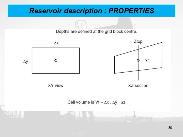
- 29. Reservoir description : PROPERTIES
- 30. Reservoir description : PROPERTIES
- 31. Reservoir Discritization Defination: the reservoir is described by a set of gridblocks (or gridpoints) whose properties,
- 32. Block Identification and Ordering
- 33. Block Identification and Ordering Natural ordering Zebra ordering Diagonal D2 ordering Alternating diagonal D4 ordering Cycle
- 34. GRID SIZE SELECTION
- 35. ACTIVE and DEAD CELLS
- 36. GEOLOGICAL CONSTRAINTS
- 37. CHOICE OF VERTICAL DISCRETIZATION
- 38. Using LGR to model gas coning
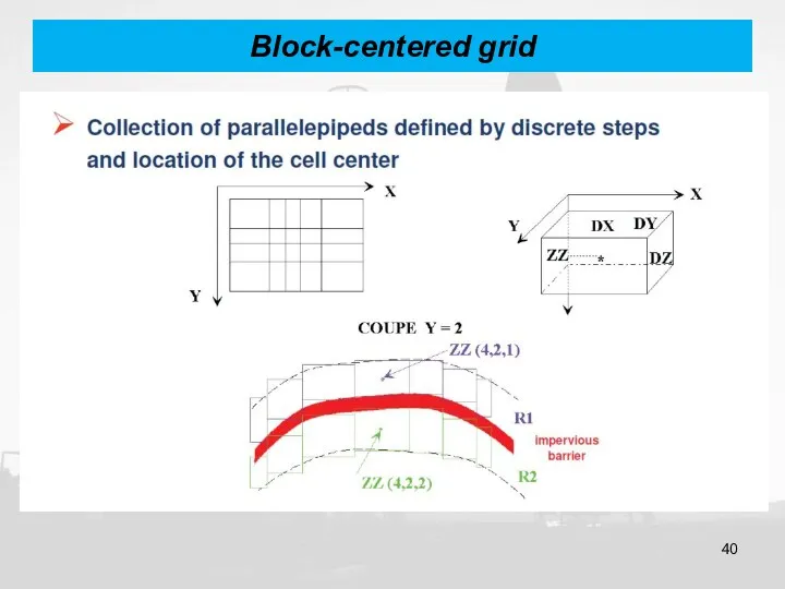
- 39. Block-centered grid
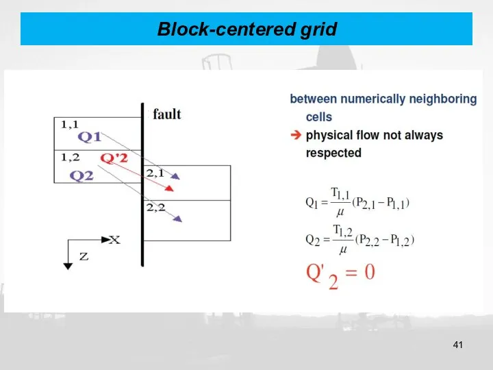
- 40. Block-centered grid
- 41. Block-centered grid
- 42. Dip or fault ?
- 43. CPG grid intercell flow
- 44. Fault description in CPG grid
- 45. Example of CPG reservoir model
- 46. Fault description in CPG grid
- 47. Reservoir layering: Use of log Correlation K.FEKI
- 48. Upscaling Optimum level of and techniques for upscaling to minimize errors Gurpinar, 2001
- 49. Rock properties: Main parameters
- 50. Rock properties: Net thickness and porosity
- 51. Rock properties: Compressibility
- 52. Rock properties: Compressibility
- 53. Horizontal & Vertical Permeability
- 54. Horizontal Permeability
- 55. Vertical Permeability
- 56. History Matching
- 57. History Matching
- 58. History Matching
- 59. FIRST STEP - GENERAL FIELD MATCH - RUN 1
- 60. FINAL STEP - GENERAL FIELD MATCH - RUN 3
- 61. Predictions
- 62. Predictions
- 63. Predictions
- 64. Fluid flow equations Conservation laws Conservation in mass Assume: Isothermal condition complete and instantaneous phase equilibration
- 65. Fluid flow equations Type of fluid in the reservoir Flow regimes Reservoir geometry Number of flowing
- 66. Type of fluid in the reservoir Incompressible Slightly compressible Compressible
- 67. Flow regimes Steady State flow Unsteady State flow Pseudo Steady State flow
- 68. Reservoir geometry Radial flow Linear flow Spherical and Hemispherical flow
- 69. Number of flowing fluids in the reservoir Single Phase flow Two phase flow Three phase flow
- 70. IN OUT Reservoir Simulator Pressure Saturation Newton-Raphson (IMPLICIT) all primary variables are calculated at the same
- 71. Numerical Models Black oil model Depletion Water Injection Component: oil water gas Phase: Oil water gas
- 72. Gas injection to increase or maintain reservoir pressure Miscible flooding as the injection gas goes into
- 73. Polymer and surfactant injection Component: Water oil surfactant alcohol Phase: Agues oleic microemulsion Chemical model
- 74. Reservoir simulators ECLIPSE GPRS SENSOR NEXUS UTCHEM Boast 3 COMET3 … Objective Accuracy Time Limitations User
- 75. Commercial reservoir simulator for over 25 years Black-oil Compositional Thermal Streamline Eclipse reservoir simulator
- 76. Eclipse reservoir simulator Local Grid Refinement Gas Lift Optimization Gas Field Operations Gas Calorific Value-Based Control
- 77. Grid definition : Example
- 78. Rock properties: Main parameters
- 79. Thank You!
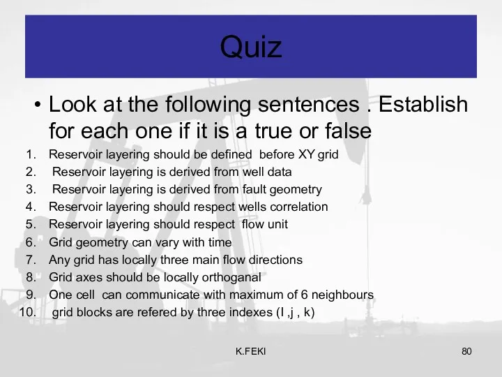
- 80. Quiz Look at the following sentences . Establish for each one if it is a true
- 81. Reservoir layering: Quiz
- 83. Скачать презентацию
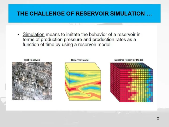
THE CHALLENGE OF RESERVOIR SIMULATION …
THE CHALLENGE OF RESERVOIR SIMULATION …
DYNAMIC RESERVOIR SIMULATION
DYNAMIC RESERVOIR SIMULATION
Incentives for running a flow simulation
Incentives for running a flow simulation
Computer Modeling
The reservoir model Fluid flow Equation within the reservoir
Computer Modeling
The reservoir model Fluid flow Equation within the reservoir
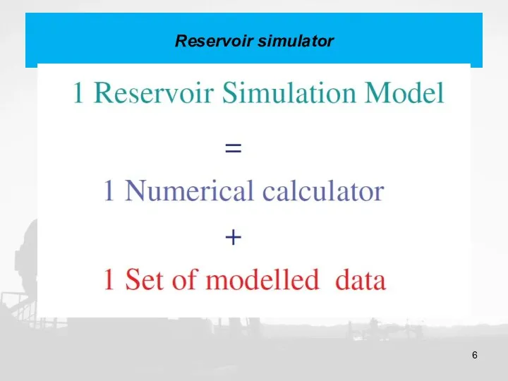
Reservoir simulator
Reservoir simulator
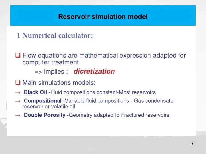
Reservoir simulation model
Reservoir simulation model
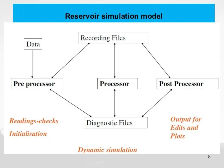
Reservoir simulation model
Reservoir simulation model
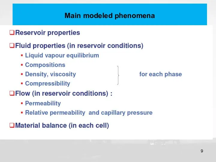
Main modeled phenomena
Main modeled phenomena
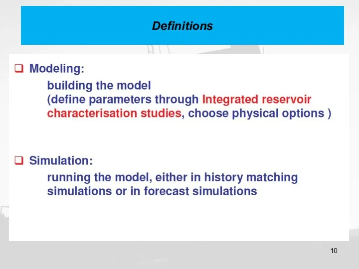
Definitions
Definitions
Types of models
Types of models
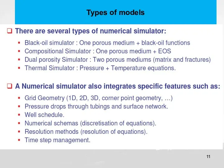
Types of simulators
Types of simulators
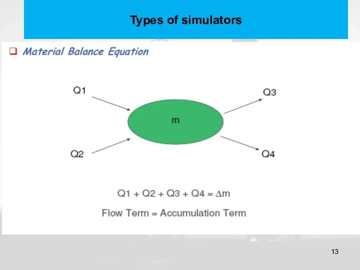
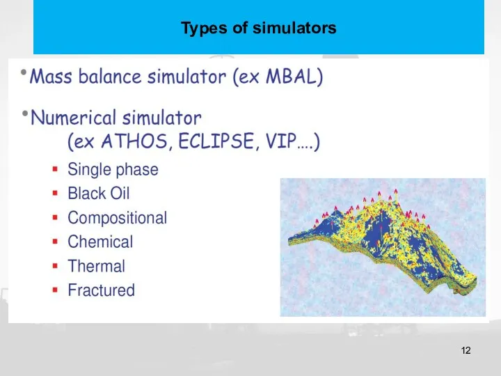
Types of simulators
Types of simulators
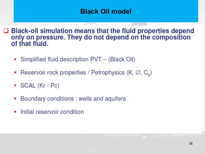
Black Oil model
Black Oil model
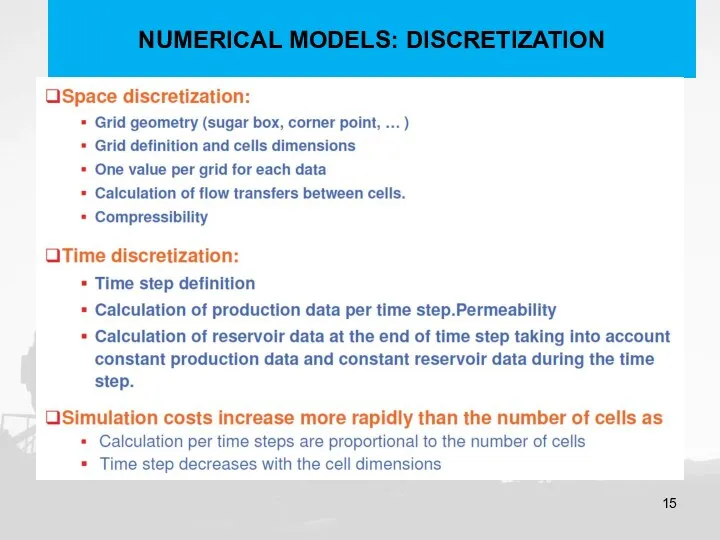
NUMERICAL MODELS: DISCRETIZATION
NUMERICAL MODELS: DISCRETIZATION
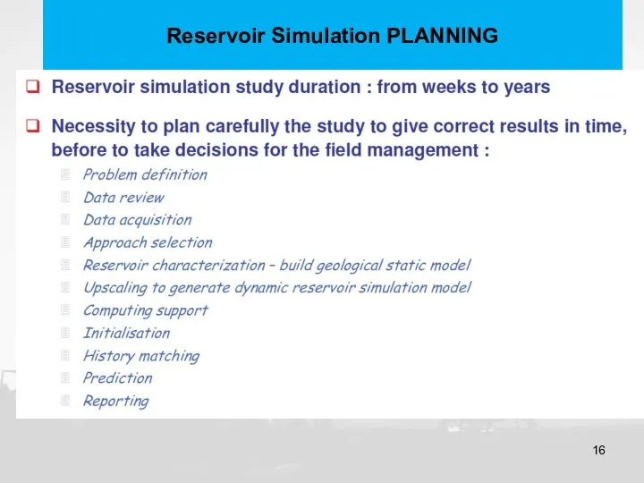
Reservoir Simulation PLANNING
Reservoir Simulation PLANNING
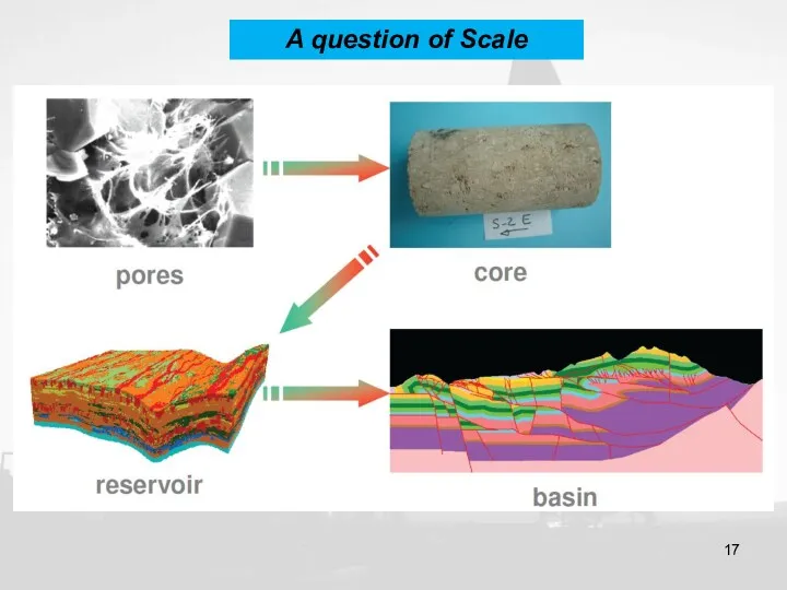
A question of Scale
A question of Scale
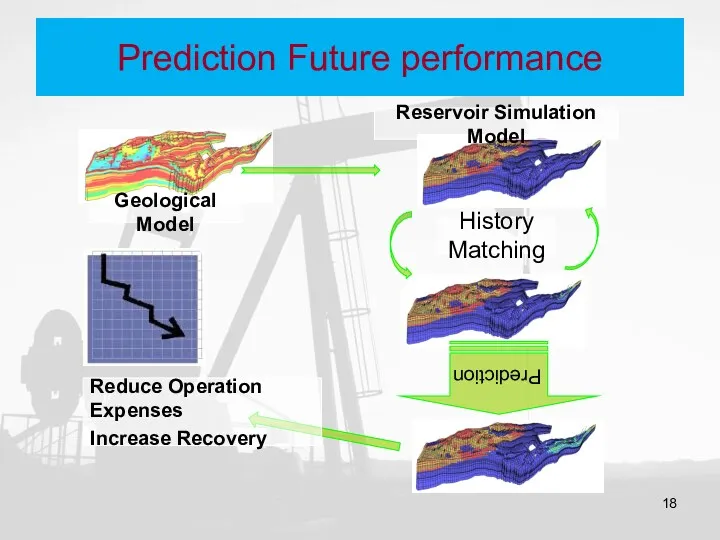
Prediction Future performance
Prediction Future performance
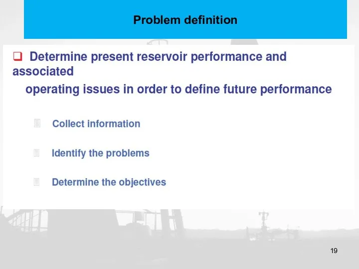
Problem definition
Problem definition
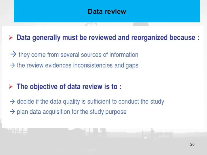
Data review
Data review
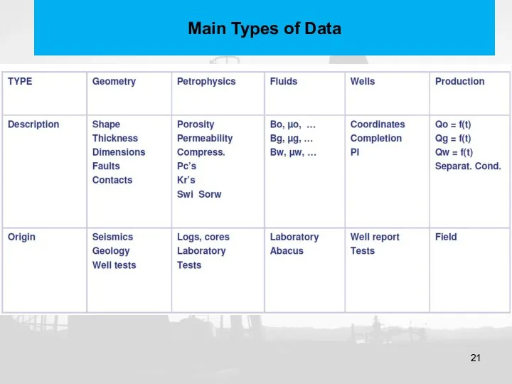
Main Types of Data
Main Types of Data
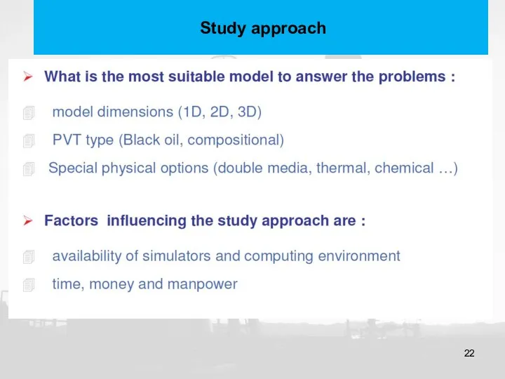
Study approach
Study approach
Study approach
Study approach
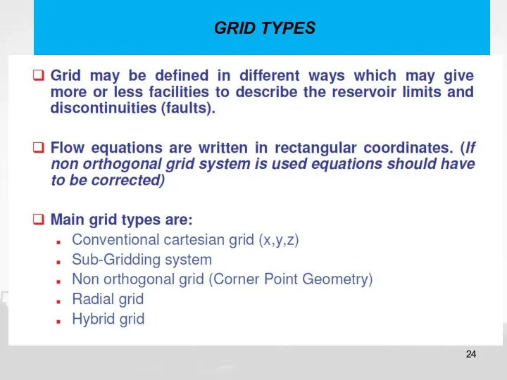
GRID TYPES
GRID TYPES
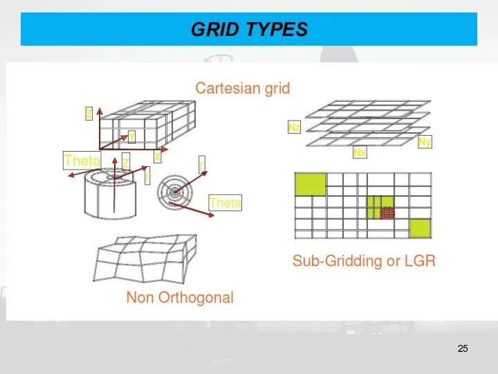
GRID TYPES
GRID TYPES
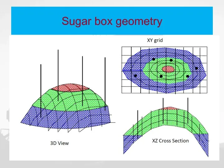
Sugar box geometry
Sugar box geometry
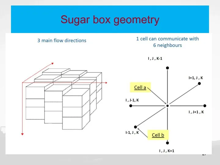
Sugar box geometry
Sugar box geometry
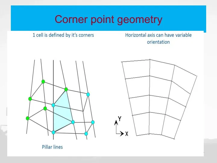
Corner point geometry
Corner point geometry
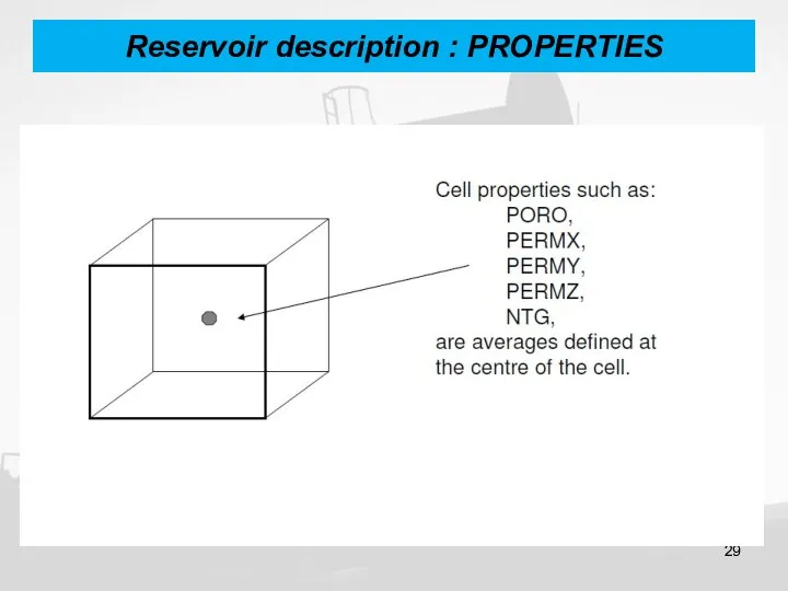
Reservoir description : PROPERTIES
Reservoir description : PROPERTIES
Reservoir description : PROPERTIES
Reservoir description : PROPERTIES
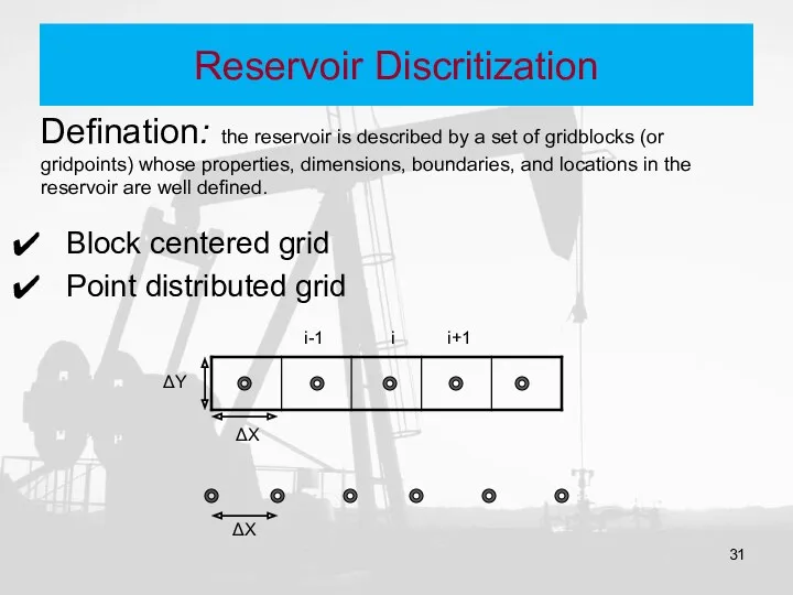
Reservoir Discritization
Defination: the reservoir is described by a set of gridblocks
Reservoir Discritization
Defination: the reservoir is described by a set of gridblocks
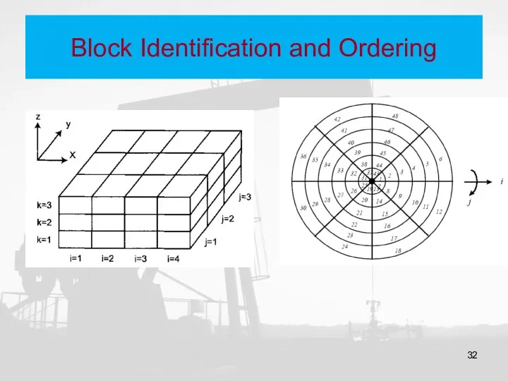
Block Identification and Ordering
Block Identification and Ordering
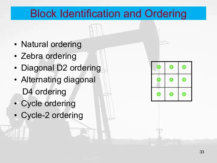
Block Identification and Ordering
Natural ordering
Zebra ordering
Diagonal D2 ordering
Alternating diagonal
Block Identification and Ordering
Natural ordering
Zebra ordering
Diagonal D2 ordering
Alternating diagonal
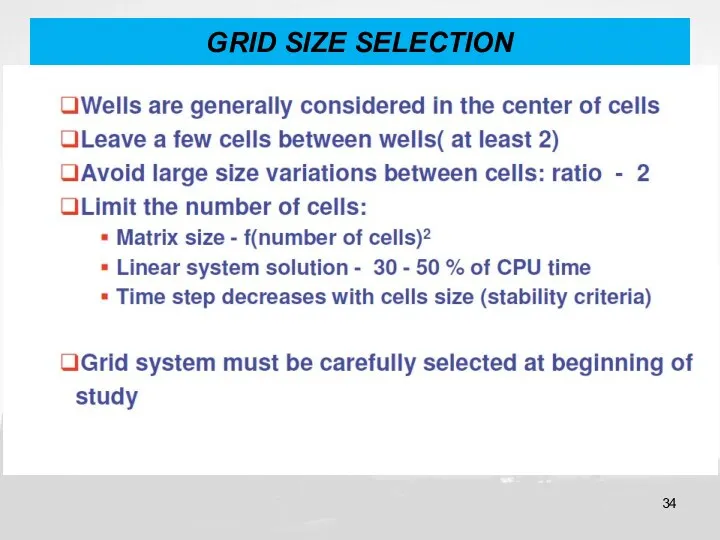
GRID SIZE SELECTION
GRID SIZE SELECTION
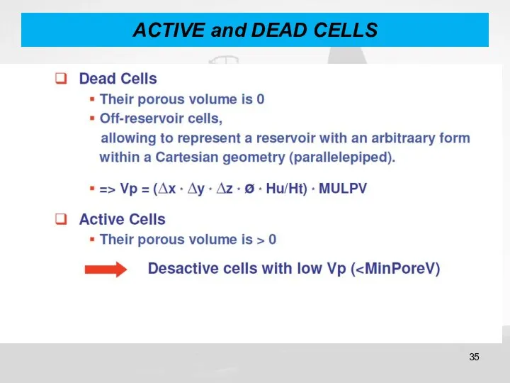
ACTIVE and DEAD CELLS
ACTIVE and DEAD CELLS
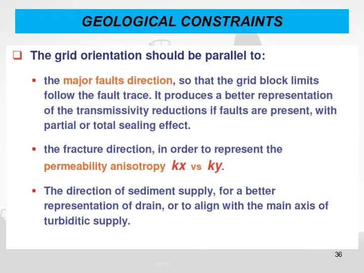
GEOLOGICAL CONSTRAINTS
GEOLOGICAL CONSTRAINTS
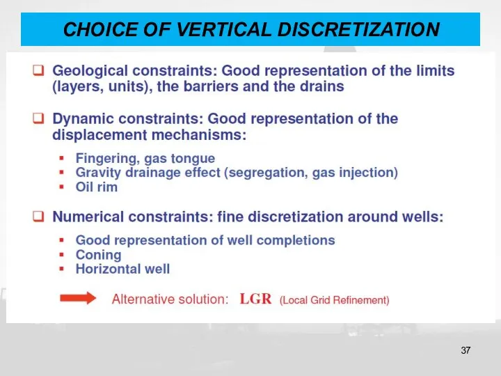
CHOICE OF VERTICAL DISCRETIZATION
CHOICE OF VERTICAL DISCRETIZATION
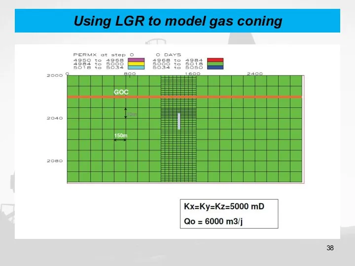
Using LGR to model gas coning
Using LGR to model gas coning

Block-centered grid
Block-centered grid
Block-centered grid
Block-centered grid
Block-centered grid
Block-centered grid
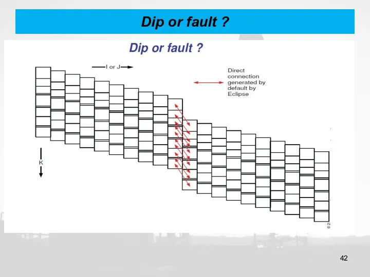
Dip or fault ?
Dip or fault ?
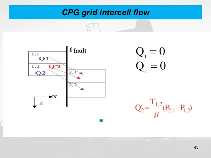
CPG grid intercell flow
CPG grid intercell flow
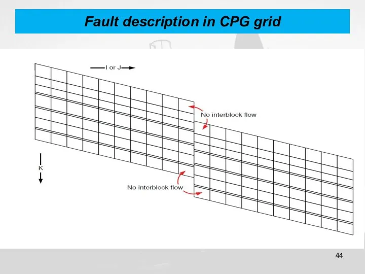
Fault description in CPG grid
Fault description in CPG grid
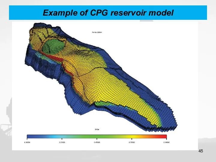
Example of CPG reservoir model
Example of CPG reservoir model
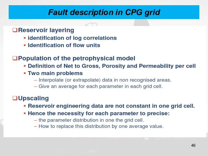
Fault description in CPG grid
Fault description in CPG grid
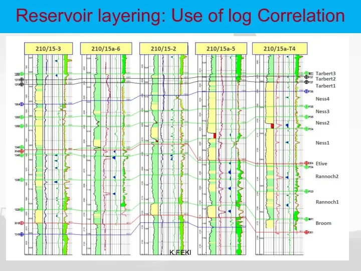
Reservoir layering: Use of log Correlation
K.FEKI
Reservoir layering: Use of log Correlation
K.FEKI
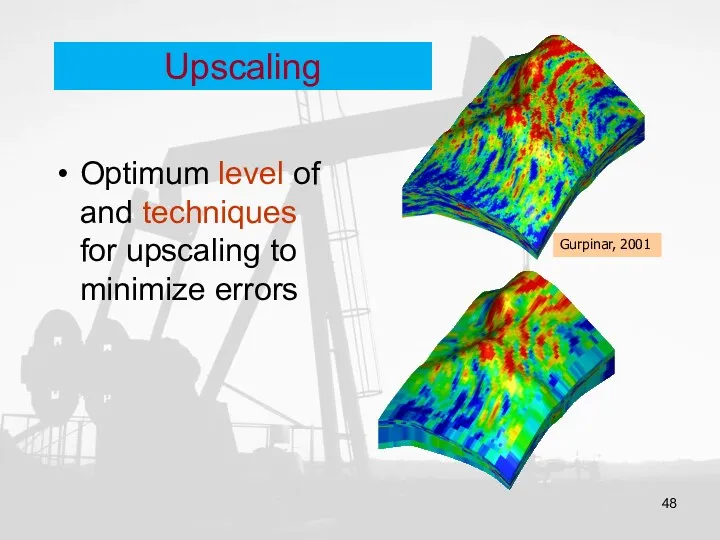
Upscaling
Optimum level of and techniques for upscaling to minimize errors
Gurpinar, 2001
Upscaling
Optimum level of and techniques for upscaling to minimize errors
Gurpinar, 2001
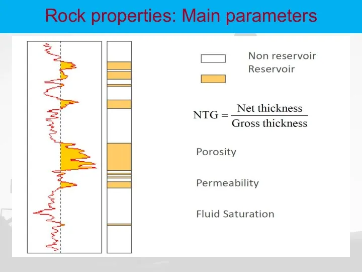
Rock properties: Main parameters
Rock properties: Main parameters
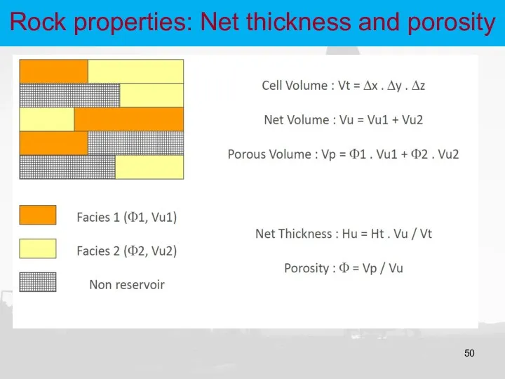
Rock properties: Net thickness and porosity
Rock properties: Net thickness and porosity
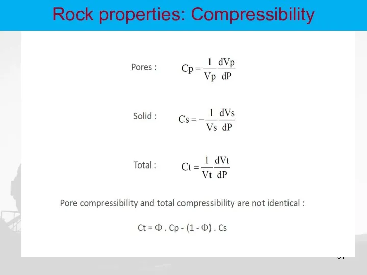
Rock properties: Compressibility
Rock properties: Compressibility
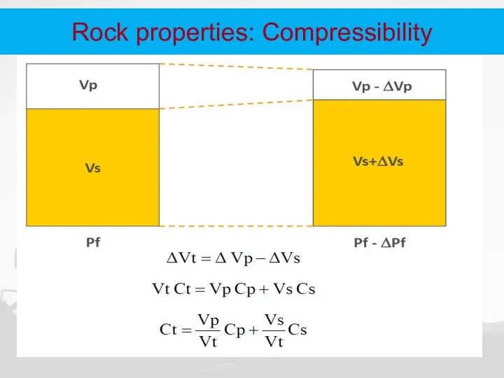
Rock properties: Compressibility
Rock properties: Compressibility
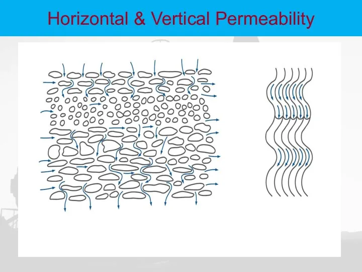
Horizontal & Vertical Permeability
Horizontal & Vertical Permeability
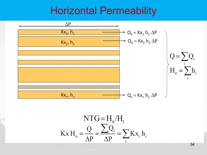
Horizontal Permeability
Horizontal Permeability
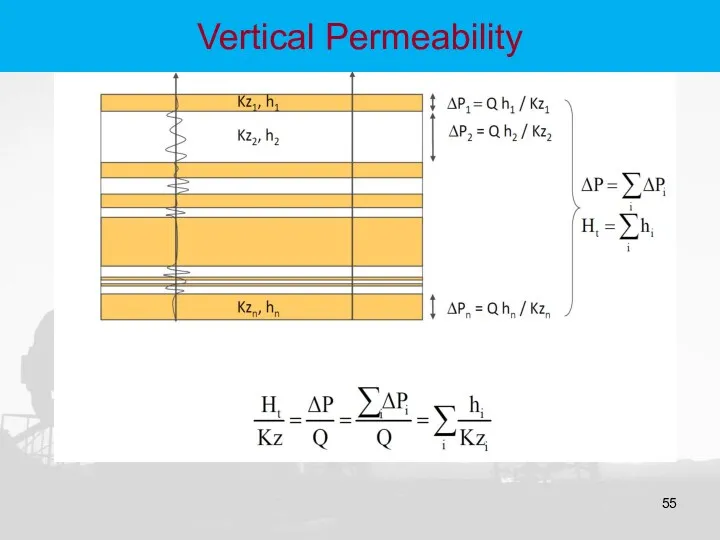
Vertical Permeability
Vertical Permeability
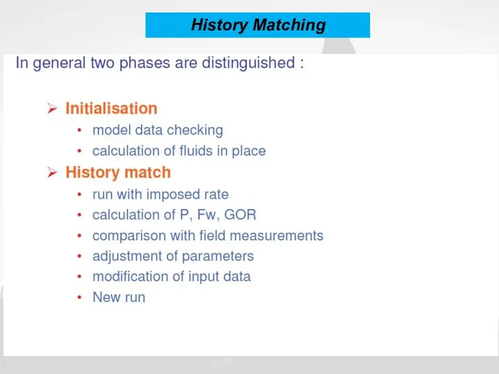
History Matching
History Matching
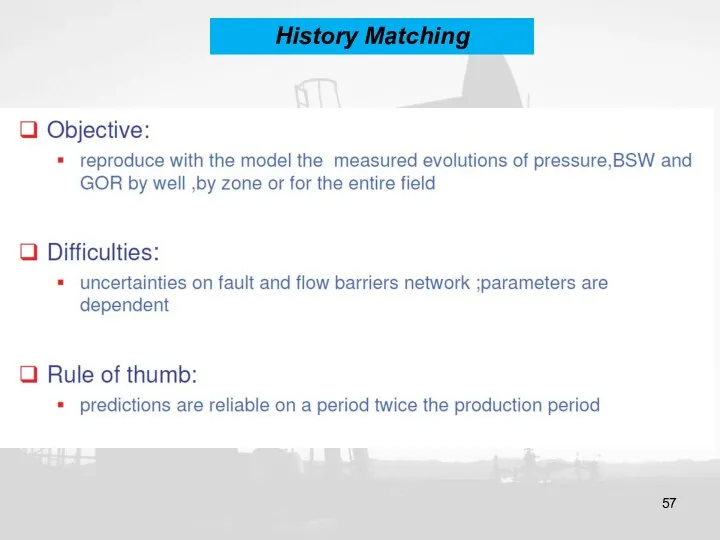
History Matching
History Matching
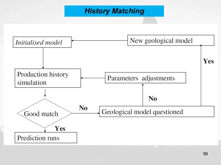
History Matching
History Matching
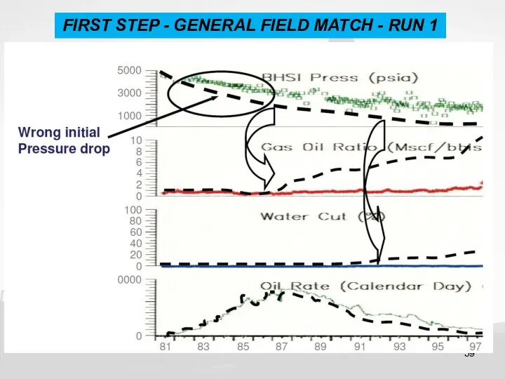
FIRST STEP - GENERAL FIELD MATCH - RUN 1
FIRST STEP - GENERAL FIELD MATCH - RUN 1
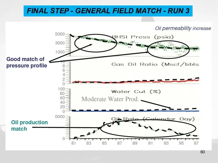
FINAL STEP - GENERAL FIELD MATCH - RUN 3
FINAL STEP - GENERAL FIELD MATCH - RUN 3
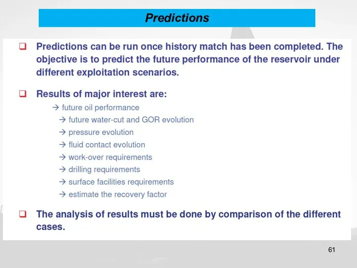
Predictions
Predictions
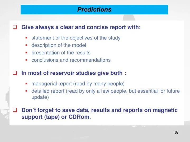
Predictions
Predictions
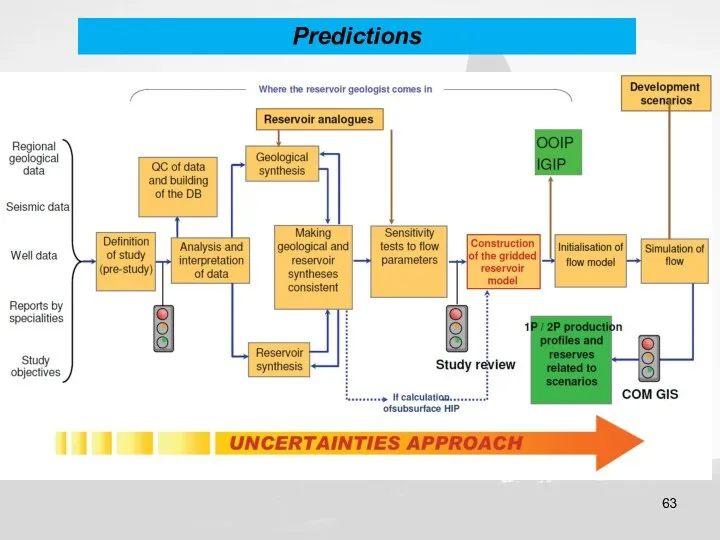
Predictions
Predictions
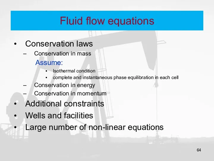
Fluid flow equations
Conservation laws
Conservation in mass
Assume:
Isothermal condition
complete and instantaneous
Fluid flow equations
Conservation laws
Conservation in mass
Assume:
Isothermal condition
complete and instantaneous
Fluid flow equations
Type of fluid in the reservoir
Flow regimes
Reservoir geometry
Number of
Fluid flow equations
Type of fluid in the reservoir
Flow regimes
Reservoir geometry
Number of
Type of fluid in the reservoir
Incompressible
Slightly compressible
Compressible
Type of fluid in the reservoir
Incompressible
Slightly compressible
Compressible
Flow regimes
Steady State flow
Unsteady State flow
Pseudo Steady State flow
Flow regimes
Steady State flow
Unsteady State flow
Pseudo Steady State flow
Reservoir geometry
Radial flow
Linear flow
Spherical and Hemispherical flow
Reservoir geometry
Radial flow
Linear flow
Spherical and Hemispherical flow
Number of flowing fluids in the reservoir
Single Phase flow
Two phase flow
Three
Number of flowing fluids in the reservoir
Single Phase flow
Two phase flow
Three
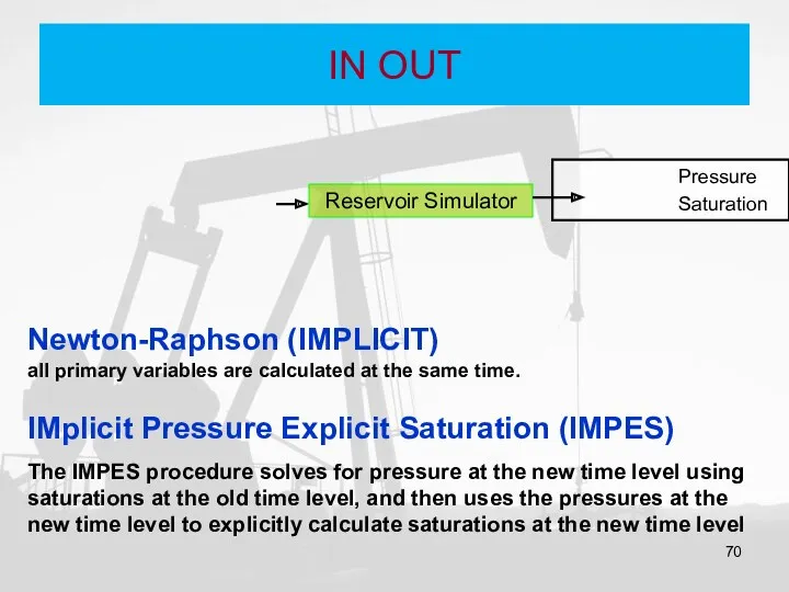
IN OUT
Reservoir Simulator
Pressure
Saturation
Newton-Raphson (IMPLICIT)
all primary variables are calculated at the same
IN OUT
Reservoir Simulator
Pressure
Saturation
Newton-Raphson (IMPLICIT)
all primary variables are calculated at the same
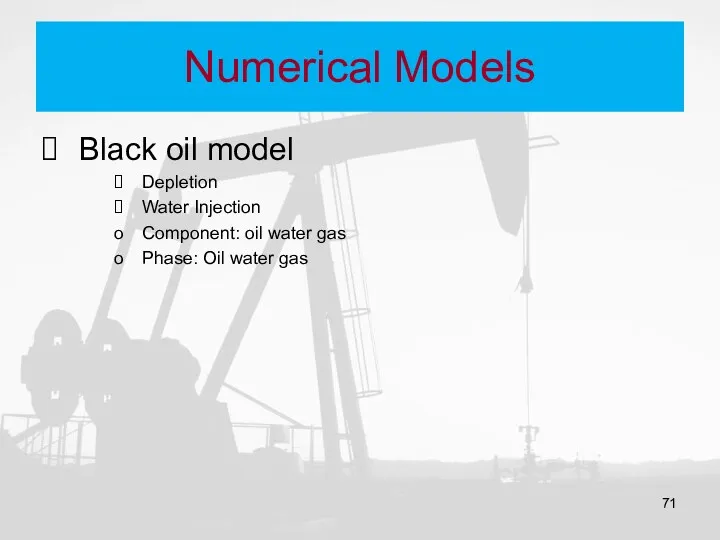
Numerical Models
Black oil model
Depletion
Water Injection
Component: oil water gas
Phase: Oil
Numerical Models
Black oil model
Depletion
Water Injection
Component: oil water gas
Phase: Oil
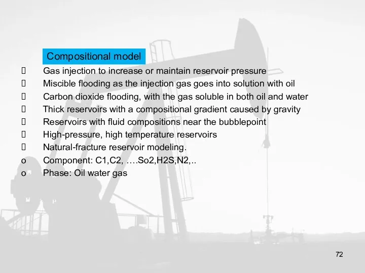
Gas injection to increase or maintain reservoir pressure
Miscible flooding
Gas injection to increase or maintain reservoir pressure
Miscible flooding
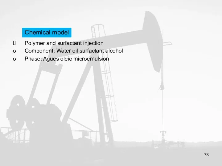
Polymer and surfactant injection
Component: Water oil surfactant alcohol
Phase:
Polymer and surfactant injection
Component: Water oil surfactant alcohol
Phase:
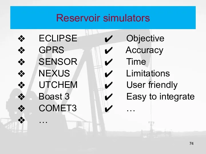
Reservoir simulators
ECLIPSE
GPRS
SENSOR
NEXUS
UTCHEM
Boast 3
Reservoir simulators
ECLIPSE
GPRS
SENSOR
NEXUS
UTCHEM
Boast 3
Commercial reservoir simulator for over 25 years
Black-oil
Compositional
Thermal
Streamline
Eclipse
Commercial reservoir simulator for over 25 years
Black-oil
Compositional
Thermal
Streamline
Eclipse
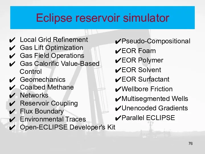
Eclipse reservoir simulator
Local Grid Refinement
Gas Lift Optimization
Gas Field Operations
Eclipse reservoir simulator
Local Grid Refinement
Gas Lift Optimization
Gas Field Operations
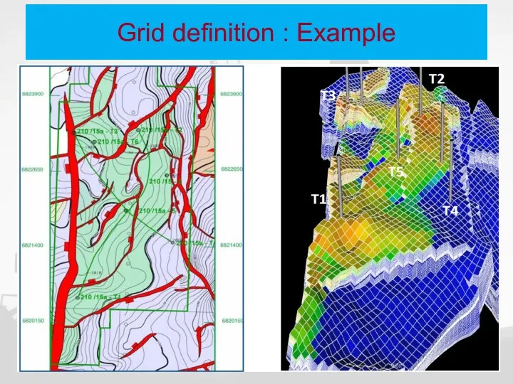
Grid definition : Example
Grid definition : Example
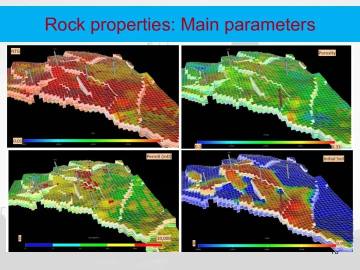
Rock properties: Main parameters
Rock properties: Main parameters

Thank You!
Thank You!
Quiz
Look at the following sentences . Establish for each one
Quiz
Look at the following sentences . Establish for each one
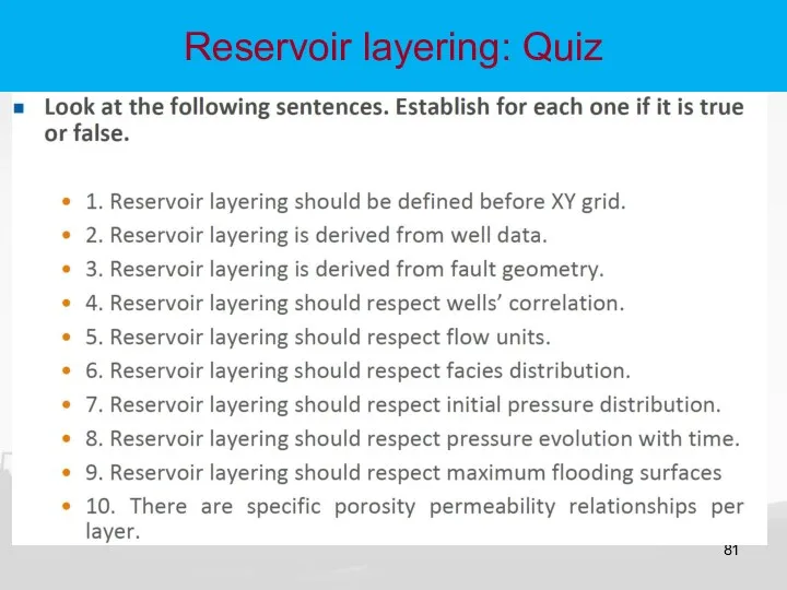
Reservoir layering: Quiz
Reservoir layering: Quiz
 Верхний рыхлый слой земли почва
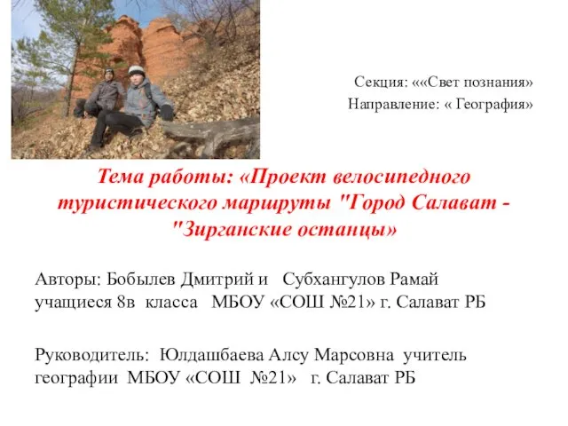 Проект велосипедного туристического маршруты Город Салават Зирганские останцы
 Общие сведения.Россия
 Этнический туризм
 Ледники. Снеговая линия. Разновидности ледников
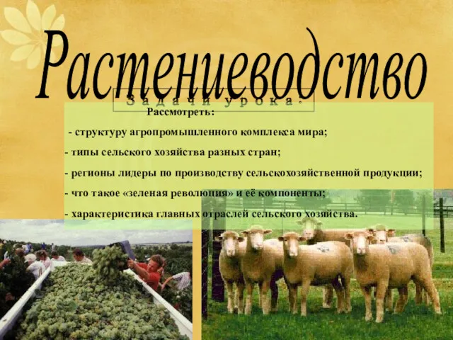 Растениеводство. Структура агропромышленного комплекса мира
 Астана қаласының жер ресурстарына мониторинг
 Факторы размещения производства
 Germany. Country in Europe
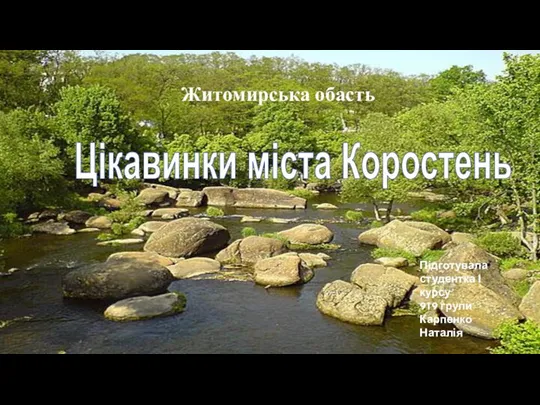 Житомирська область. Цікавинка міста Коростень
 Географический парад знаний (7 класс)
 Африка
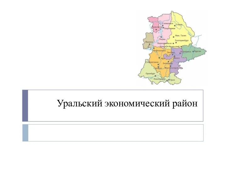 Уральский экономический район
 Япония – страна восходящего солнца
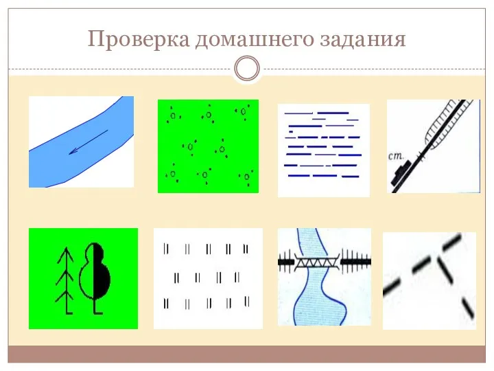 Масштаб
 Почвообразующие породы и почвы Беларуси
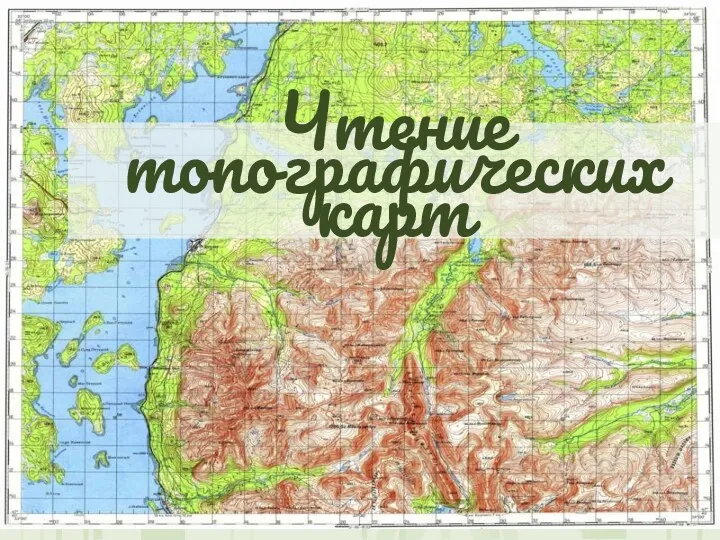 Чтение топографических карт
 The Swiss Confederation
 Страны мира Россия. Всё о России
 Мировой океан и его свойства
 Садонское (Pb-Zn) месторождение
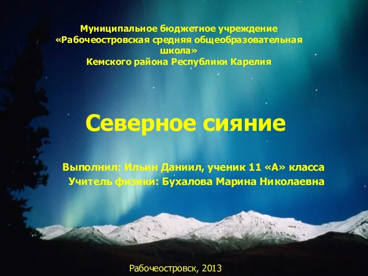 Северное сияние
 География как наука. Ее роль и значение в системе наук
 Презентация по географии Австралия
 Мой родной край - Солнечная Долина
 Конкурс 7 чудес моего района
 Европейский Союз
 Всероссийская перепись населения 2020 года