- School of Engineering and Digital Sciences

Содержание
- 2. Section 1.3 p 1.3 Separable ODEs. Modeling
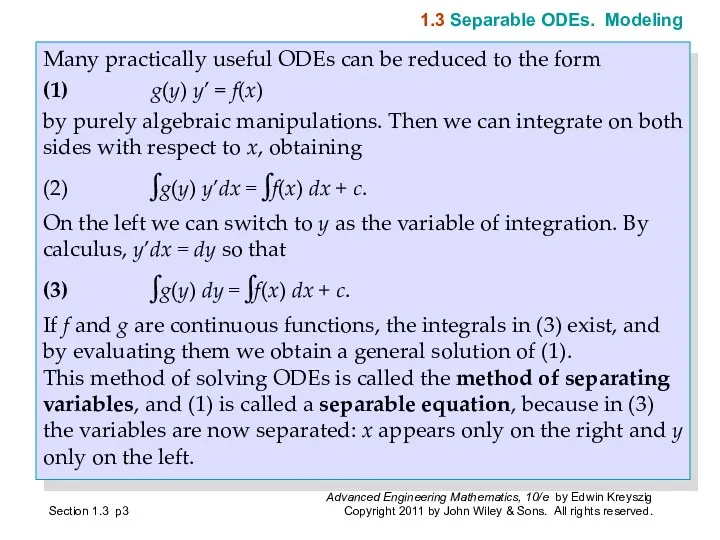
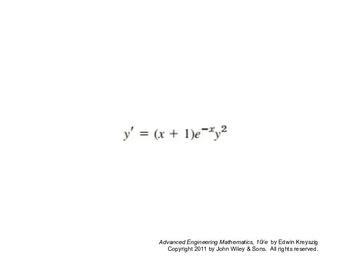
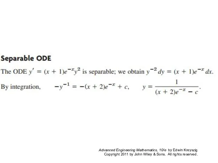
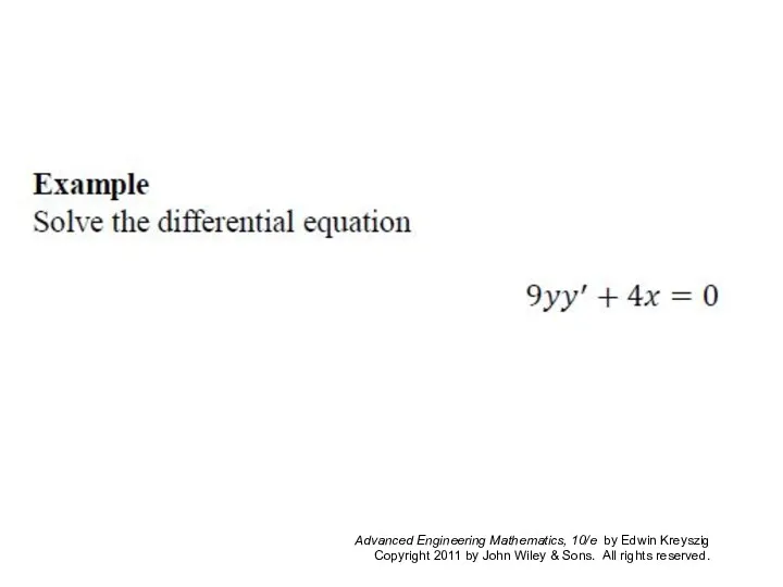
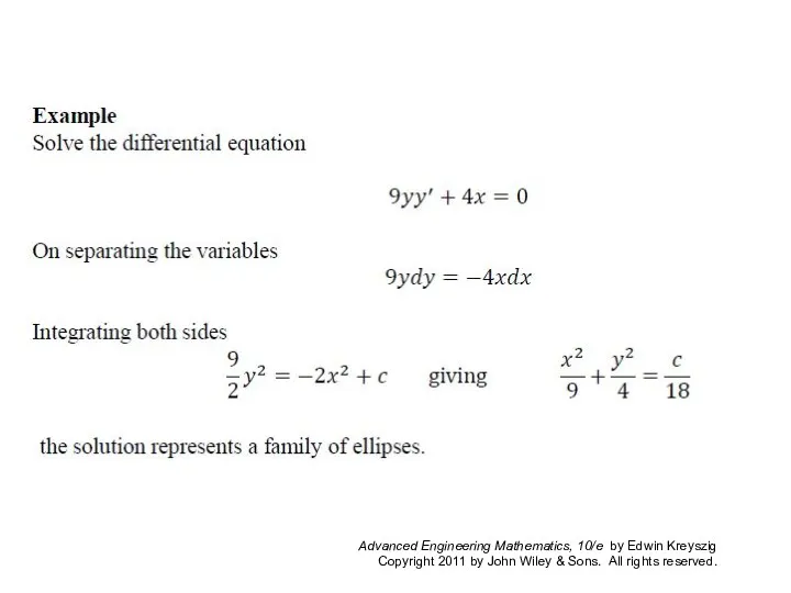
- 3. Section 1.3 p Many practically useful ODEs can be reduced to the form (1) g(y) y’
- 14. EXAMPLE 5 Mixing Problem Mixing problems occur quite frequently in chemical industry. We explain here how
- 15. EXAMPLE 5 (continued) Solution. Step 1. Setting up a model. Let y(t) denote the amount of
- 16. EXAMPLE 5 (continued) Step 2. Solution of the model. The ODE (4) is separable. Separation, integration,
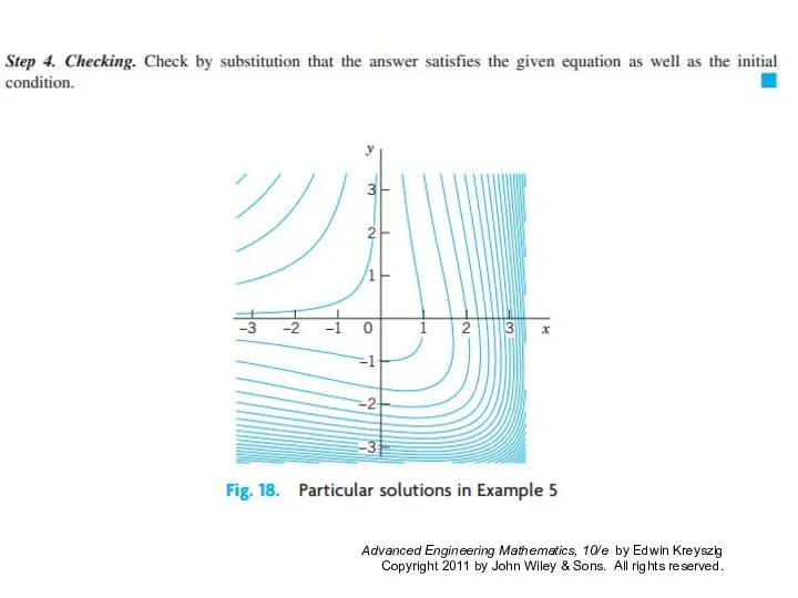
- 17. EXAMPLE 5 (continued) The model discussed becomes more realistic in problems on pollutants in lakes (see
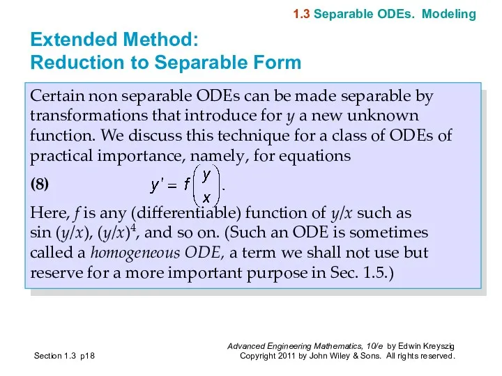
- 18. Certain non separable ODEs can be made separable by transformations that introduce for y a new
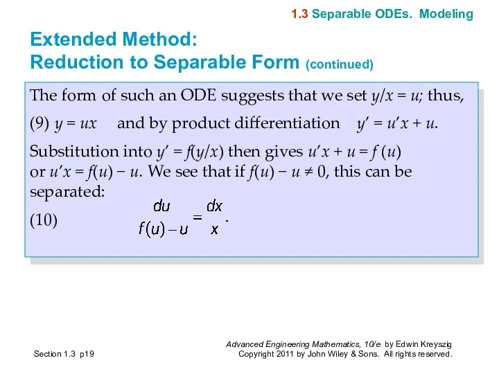
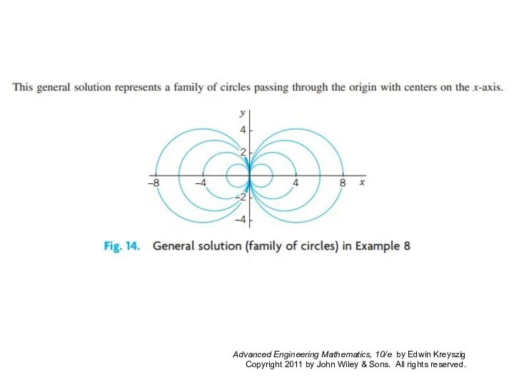
- 19. The form of such an ODE suggests that we set y/x = u; thus, (9) y
- 24. Section 1.4 p 1.4 Exact ODEs. Integrating Factors
- 25. We recall from calculus that if a function u(x, y) has continuous partial derivatives, its differential
- 26. A first-order ODE M(x, y) + N(x, y)y’ = 0, written as (use dy = y’dx
- 27. This is called an implicit solution, in contrast to a solution y = h(x) as defined
- 28. Let M and N be continuous and have continuous first partial derivatives in a region in
- 29. This condition is not only necessary but also sufficient for (1) to be an exact differential
- 31. Example
- 36. We multiply a given nonexact equation, (12) P(x, y) dx + Q(x, y) dy = 0,
- 37. For M dx + N dy = 0 the exactness condition (5) is ∂M/∂y = ∂N/∂x.
- 38. Let F = F(x). Then Fy = 0, and Fx = F’ = dF/dx, so that
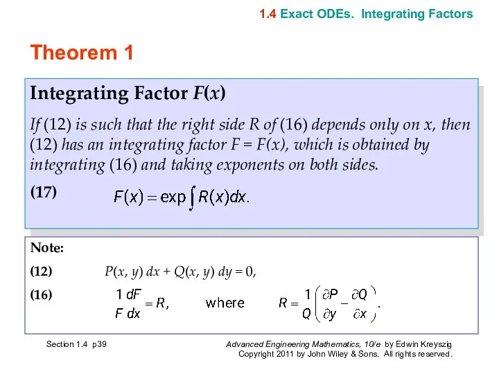
- 39. Section 1.4 p Theorem 1 Integrating Factor F(x) If (12) is such that the right side
- 40. Similarly, if F* = F*(y), then instead of (16) we get (18) Section 1.4 p 1.4
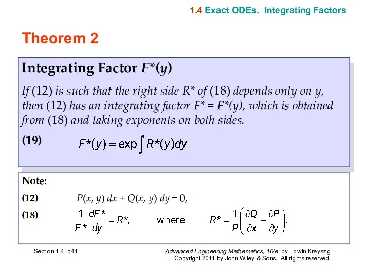
- 41. Section 1.4 p Theorem 2 Integrating Factor F*(y) If (12) is such that the right side
- 50. Section 1.5 p 1.5 Linear ODEs. Bernoulli Equation. Population Dynamics
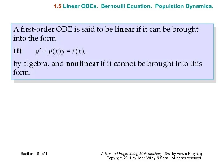
- 51. A first-order ODE is said to be linear if it can be brought into the form
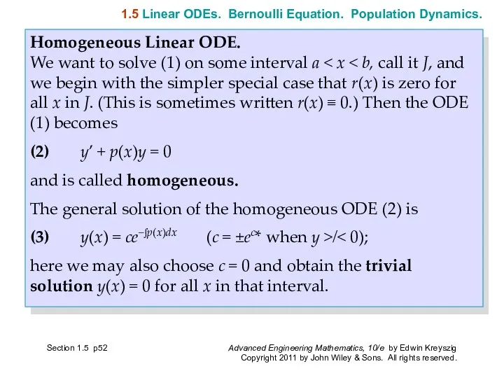
- 52. Homogeneous Linear ODE. We want to solve (1) on some interval a (2) y’ + p(x)y
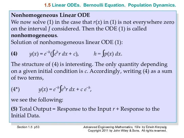
- 53. Nonhomogeneous Linear ODE We now solve (1) in the case that r(x) in (1) is not
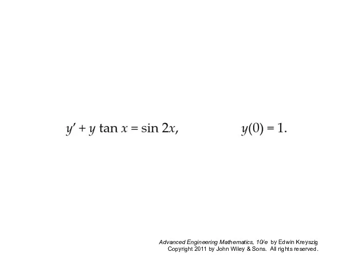
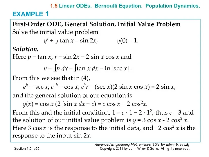
- 55. EXAMPLE 1 First-Order ODE, General Solution, Initial Value Problem Solve the initial value problem y’ +
- 56. Numerous applications can be modeled by ODEs that are nonlinear but can be transformed to linear
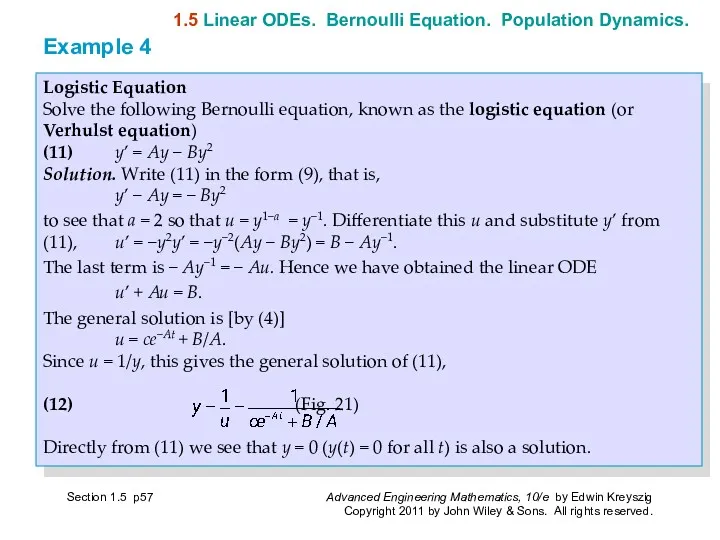
- 57. Logistic Equation Solve the following Bernoulli equation, known as the logistic equation (or Verhulst equation) (11)
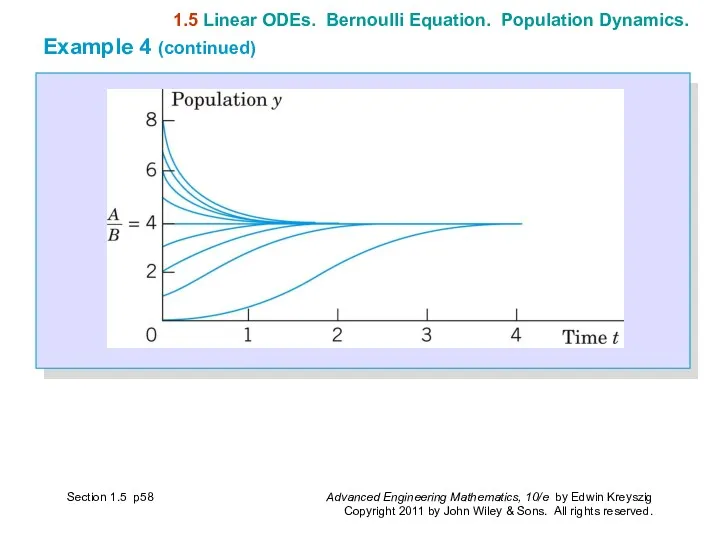
- 58. 1.5 Linear ODEs. Bernoulli Equation. Population Dynamics. Section 1.5 p Example 4 (continued)
- 59. SUMMARY OF CHAPTER 1 First-Order ODEs Section 1.Summary p
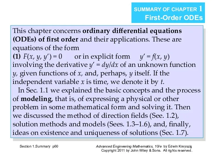
- 60. Section 1.Summary p SUMMARY OF CHAPTER 1 First-Order ODEs This chapter concerns ordinary differential equations (ODEs)
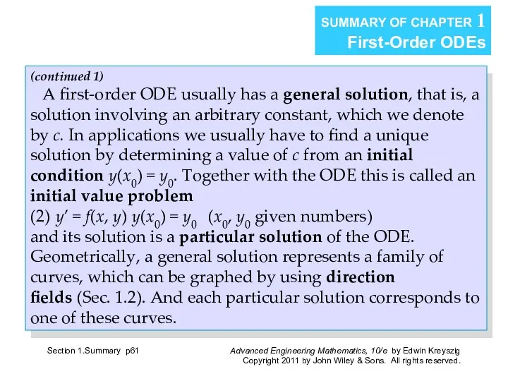
- 61. Section 1.Summary p SUMMARY OF CHAPTER 1 First-Order ODEs (continued 1) A first-order ODE usually has
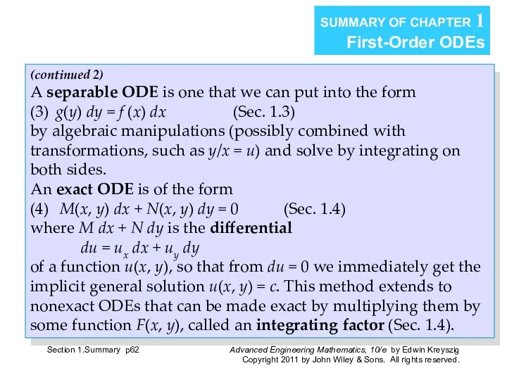
- 62. Section 1.Summary p SUMMARY OF CHAPTER 1 First-Order ODEs (continued 2) A separable ODE is one
- 64. Скачать презентацию
Section 1.3 p
1.3 Separable ODEs. Modeling
Section 1.3 p
1.3 Separable ODEs. Modeling
Section 1.3 p
Many practically useful ODEs can be reduced to the
Section 1.3 p
Many practically useful ODEs can be reduced to the
EXAMPLE 5
Mixing Problem
Mixing problems occur quite frequently in chemical industry. We
EXAMPLE 5
Mixing Problem
Mixing problems occur quite frequently in chemical industry. We
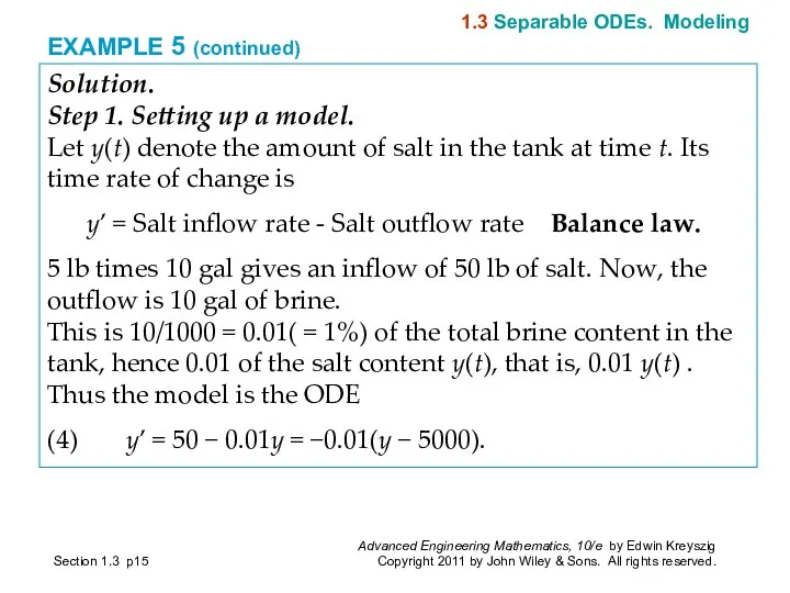
EXAMPLE 5 (continued)
Solution.
Step 1. Setting up a model.
Let y(t)
EXAMPLE 5 (continued)
Solution.
Step 1. Setting up a model.
Let y(t)
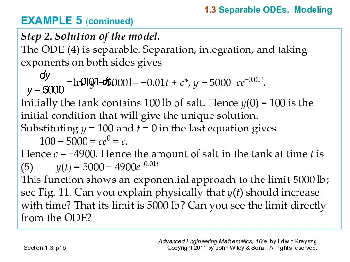
EXAMPLE 5 (continued)
Step 2. Solution of the model.
The ODE (4)
EXAMPLE 5 (continued)
Step 2. Solution of the model.
The ODE (4)
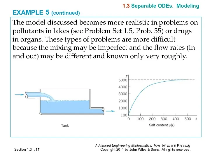
EXAMPLE 5 (continued)
The model discussed becomes more realistic in problems on
EXAMPLE 5 (continued)
The model discussed becomes more realistic in problems on
Certain non separable ODEs can be made separable by transformations that
Certain non separable ODEs can be made separable by transformations that
The form of such an ODE suggests that we set y/x
The form of such an ODE suggests that we set y/x
Section 1.4 p
1.4 Exact ODEs. Integrating Factors
Section 1.4 p
1.4 Exact ODEs. Integrating Factors
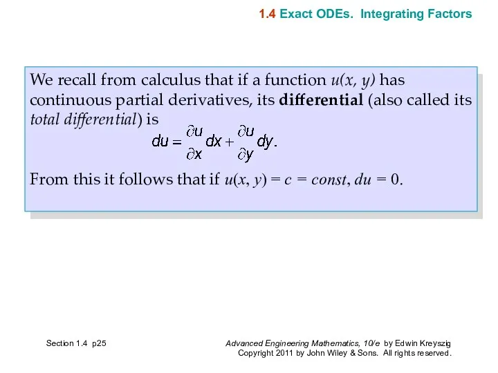
We recall from calculus that if a function u(x, y) has
We recall from calculus that if a function u(x, y) has
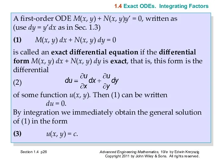
A first-order ODE M(x, y) + N(x, y)y’ = 0, written
A first-order ODE M(x, y) + N(x, y)y’ = 0, written
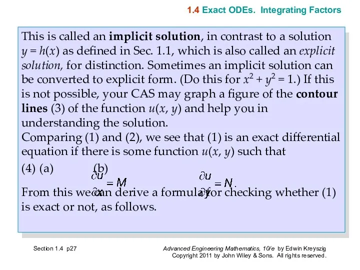
This is called an implicit solution, in contrast to a solution
This is called an implicit solution, in contrast to a solution
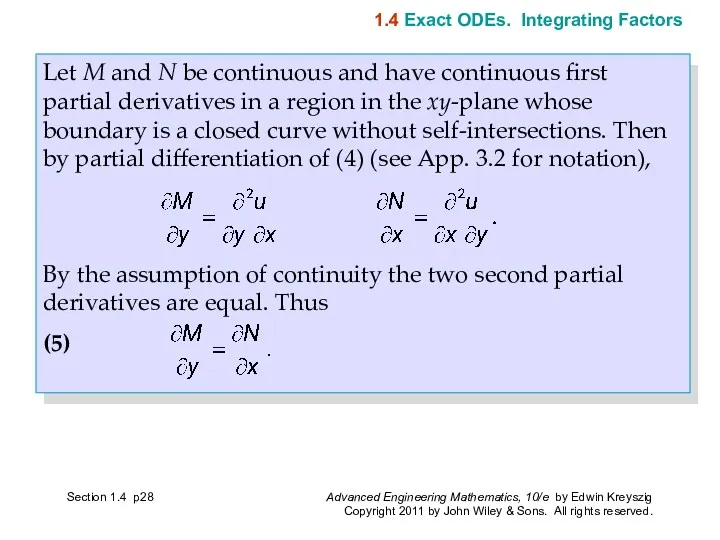
Let M and N be continuous and have continuous first partial
Let M and N be continuous and have continuous first partial
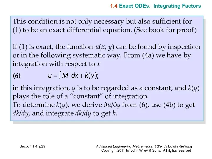
This condition is not only necessary but also sufficient for (1)
This condition is not only necessary but also sufficient for (1)
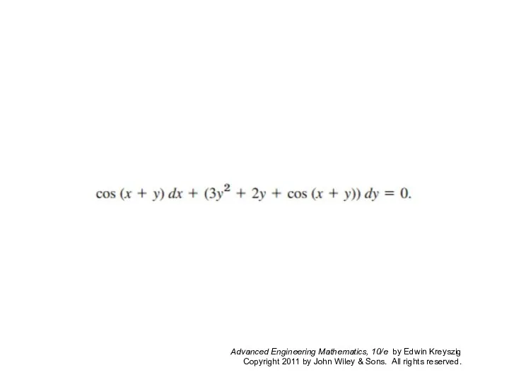
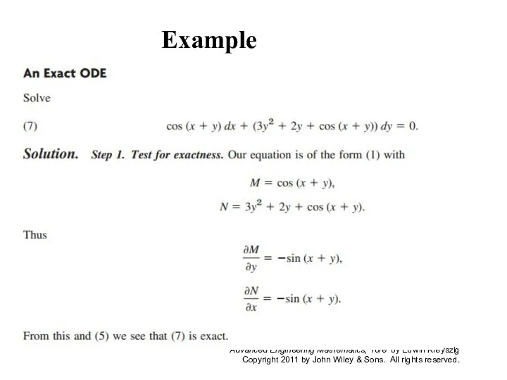
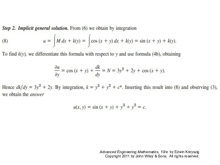
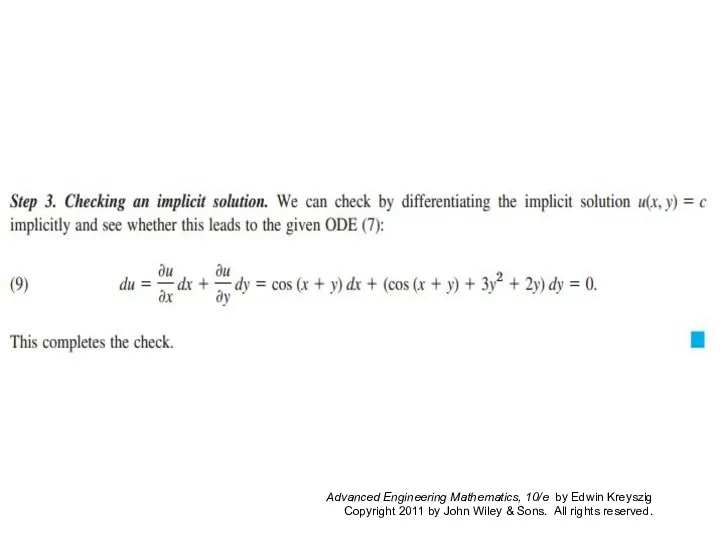
Example
Example
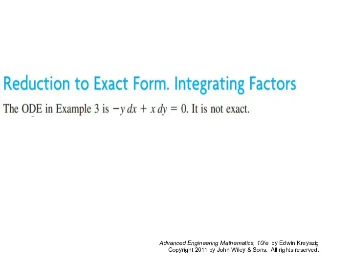
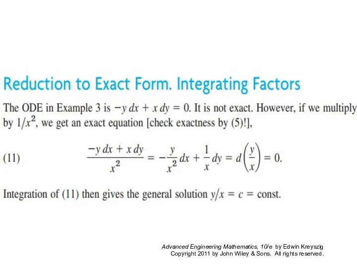
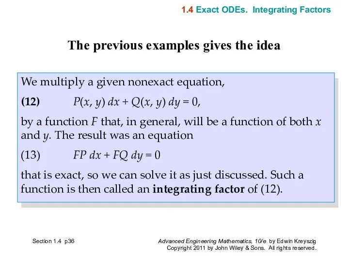
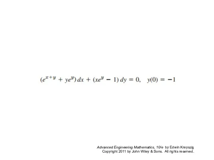
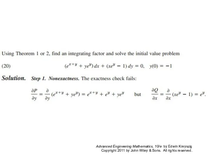
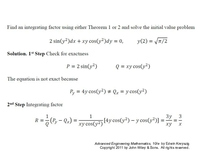
We multiply a given nonexact equation,
(12) P(x, y) dx +
We multiply a given nonexact equation,
(12) P(x, y) dx +
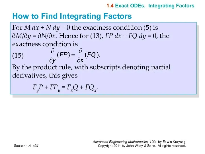
For M dx + N dy = 0 the exactness condition
For M dx + N dy = 0 the exactness condition
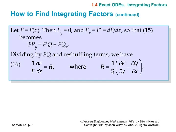
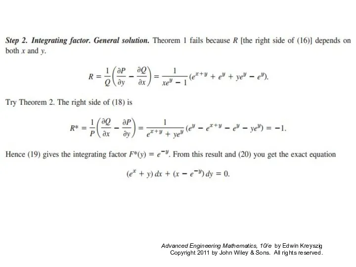
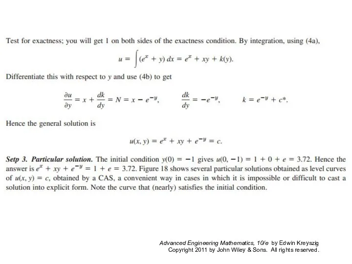
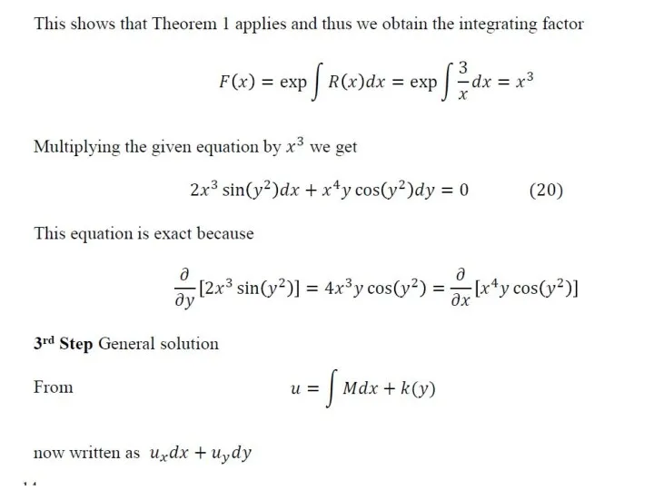
Let F = F(x). Then Fy = 0, and Fx =
Let F = F(x). Then Fy = 0, and Fx =
Section 1.4 p
Theorem 1
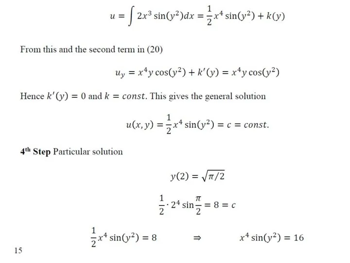
Integrating Factor F(x)
If (12) is such that the
Section 1.4 p
Theorem 1
Integrating Factor F(x)
If (12) is such that the
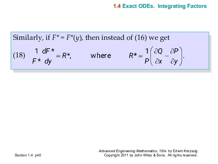
Similarly, if F* = F*(y), then instead of (16) we get
(18)
Section
Similarly, if F* = F*(y), then instead of (16) we get
(18)
Section
Section 1.4 p
Theorem 2
Integrating Factor F*(y)
If (12) is such that the
Section 1.4 p
Theorem 2
Integrating Factor F*(y)
If (12) is such that the
Section 1.5 p
1.5 Linear ODEs. Bernoulli Equation. Population Dynamics
Section 1.5 p
1.5 Linear ODEs. Bernoulli Equation. Population Dynamics
A first-order ODE is said to be linear if it can
A first-order ODE is said to be linear if it can
Homogeneous Linear ODE.
We want to solve (1) on some interval
Homogeneous Linear ODE.
We want to solve (1) on some interval
Nonhomogeneous Linear ODE
We now solve (1) in the case that r(x)
Nonhomogeneous Linear ODE
We now solve (1) in the case that r(x)
EXAMPLE 1
First-Order ODE, General Solution, Initial Value Problem
Solve the initial value
EXAMPLE 1
First-Order ODE, General Solution, Initial Value Problem
Solve the initial value
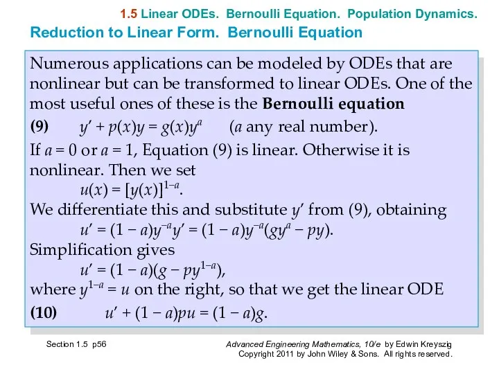
Numerous applications can be modeled by ODEs that are nonlinear but
Numerous applications can be modeled by ODEs that are nonlinear but
Logistic Equation
Solve the following Bernoulli equation, known as the logistic equation
Logistic Equation
Solve the following Bernoulli equation, known as the logistic equation
1.5 Linear ODEs. Bernoulli Equation. Population Dynamics.
Section 1.5 p
Example 4 (continued)
1.5 Linear ODEs. Bernoulli Equation. Population Dynamics.
Section 1.5 p
Example 4 (continued)
SUMMARY OF CHAPTER 1
First-Order ODEs
Section 1.Summary p
SUMMARY OF CHAPTER 1
First-Order ODEs
Section 1.Summary p
Section 1.Summary p
SUMMARY OF CHAPTER 1
First-Order ODEs
This chapter concerns ordinary differential
Section 1.Summary p
SUMMARY OF CHAPTER 1
First-Order ODEs
This chapter concerns ordinary differential
Section 1.Summary p
SUMMARY OF CHAPTER 1
First-Order ODEs
(continued 1)
A first-order ODE
Section 1.Summary p
SUMMARY OF CHAPTER 1
First-Order ODEs
(continued 1)
A first-order ODE
Section 1.Summary p
SUMMARY OF CHAPTER 1
First-Order ODEs
(continued 2)
A separable ODE is
Section 1.Summary p
SUMMARY OF CHAPTER 1
First-Order ODEs
(continued 2)
A separable ODE is
 Виртуальная экскурсия на мемориал Защитникам Ленинграда
 Московский городской конкурс исследовательских и проектных работ обучающихся
 Типы проектов. Структура индивидуального проекта
 Порядок проведения итогового сочинения (изложения) в 2019-2020 учебном году
 Итоги проведения ГИА-2016. Подготовка к государственной итоговой аттестации в 2017 году
 Презентация Самостоятельная работа на уроках русского языка
 Технология проектной деятельности: структура и содержание проекта
 Одеська Національна Академія Харчових Технологій
 Рефлексия как этап современного урока в условиях ФГОС
 Программа развития учителей будущего Next–Педагог
 Подготовка, выполнение и защита выпускной квалификационной работы
 Развитие поликультурного образования в России
 Лекция как форма обучения
 Квиз. Своя игра
 Вчимося читати
 Требования к современному уроку в рамках ФГОС
 Внедрение дополнительных общеобразовательных программ для подростков с ограниченными возможностями здоровья
 Профессиональный стандарт педагога в начальной школе
 Системно-деятельностный подход в обучении младшего школьника
 Правила оформления курсовой работы. Программирование на языке высокого уровня
 Отчет о прохождении летней практики
 Федеральные основные образовательные программы
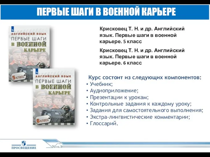 Английский язык для будущих военных
 Презентация к теме самообразования Тестирование в начальных классах как способ повышения качества обучения
 CV Writing
 О региональных проектах национального проектаОбразование
 Концепция духовно-нравственного развития и воспитания личности гражданина России (образовательная система Школа 2100)
 Президиум №16 от 29.11.2019 года Азовской организации профсоюза работников народного образования и науки РФ