- Classifying. Why a separator?

Содержание
- 2. Why a separator? Open circuit grinding is not very efficient: Overgrinding of fines Useless for quality
- 3. Closed circuit
- 4. Impact on product PSD
- 5. Impact on product PSD
- 6. Separation in general A SEPARATOR DOES NOT GRIND !!! … but it helps optimize the efficiency
- 7. Circulating Load (CL) How can we determine it? C.L. = R/F (used by Lafarge) Others define
- 8. Separation efficiency How do we assess the efficiency of separation? The tool is the separation curve,
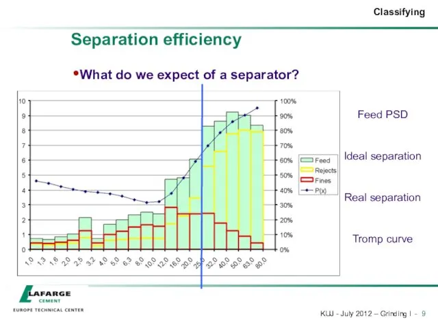
- 9. Separation efficiency What do we expect of a separator? Feed PSD Ideal separation Real separation Tromp
- 10. Tromp curve - Principle Particle size X (µm) For a given X, % of particles of
- 11. Tromp curve – example Let’s take the example of a sieve:
- 12. Tromp curve – example If screen and sieving are perfect: A F R
- 13. Tromp curve – Perfect screen 50µm Above 50 µm, all particles end up in the rejects
- 14. By-pass How can we find some fine particles in the rejects?:
- 15. Tromp curve – With bypass 50µm 20% direct by-pass
- 16. Imperfection How can we find some coarse particles in the fines?:
- 17. Tromp curve – With imperfection 50µm For particles slightly above 50 µm, a certain quantity can
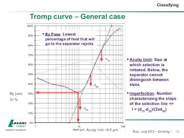
- 18. Tromp curve – General case By Pass: Lowest percentage of feed that will go to the
- 19. Tromp curve - Interpretation By-pass Should be as low as possible Directly linked to separator efficiency:
- 20. Variation of the By Pass vs CL
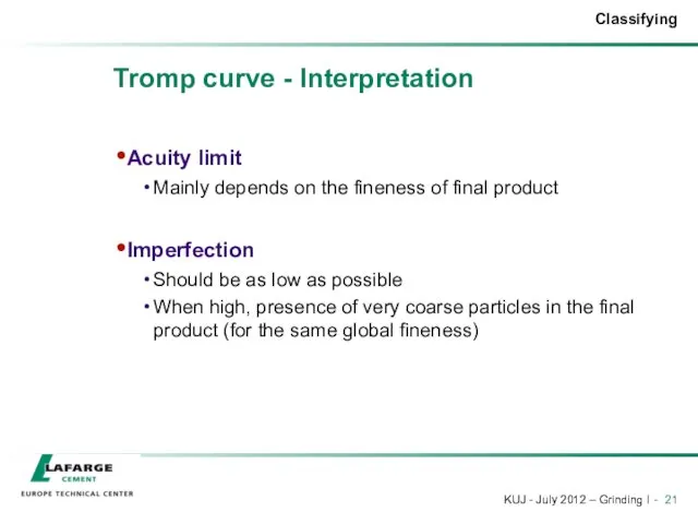
- 21. Tromp curve - Interpretation Acuity limit Mainly depends on the fineness of final product Imperfection Should
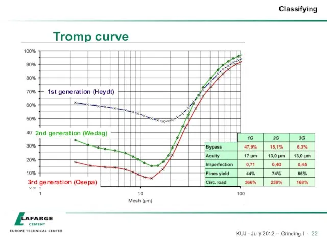
- 22. Tromp curve 1st generation (Heydt) 2nd generation (Wedag) 3rd generation (Osepa)
- 23. Typical values Tromp curve
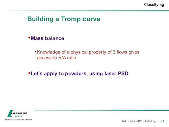
- 24. Building a Tromp curve Mass balance Knowledge of a physical property of 3 flows gives access
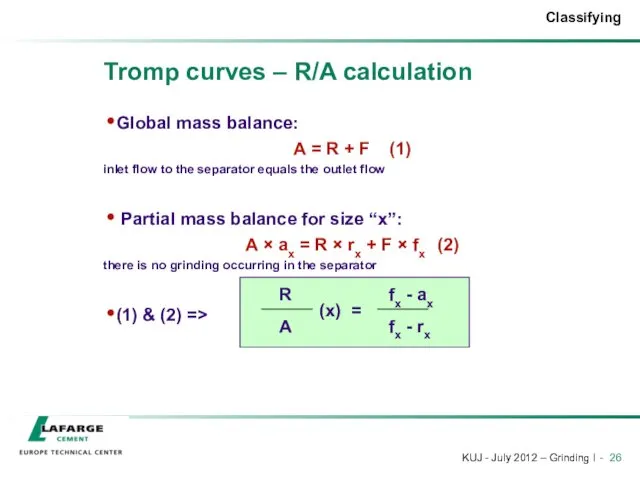
- 25. Tromp curve: notations Separator Feed Fines Rejects A = feed flow (t/h) ax = % of
- 26. Tromp curves – R/A calculation Global mass balance: A = R + F (1) inlet flow
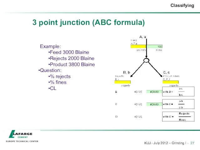
- 27. 3 point junction (ABC formula) Example: Feed 3000 Blaine Rejects 2000 Blaine Product 3800 Blaine Question:
- 28. 3 point junction (ABC formula) Example: Feed 3000 Blaine Rejects 2000 Blaine Product 3800 Blaine Question:
- 29. 3 point junction (ABC formula)
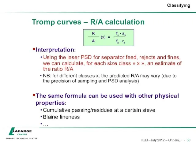
- 30. Tromp curves – R/A calculation Interpretation: Using the laser PSD for separator feed, rejects and fines,
- 31. Tromp curves – average R/A From all the values of R/A calculated before (one for each
- 32. Tromp curves – final calculation From equations (1) and (2): A = R + F and
- 34. Скачать презентацию
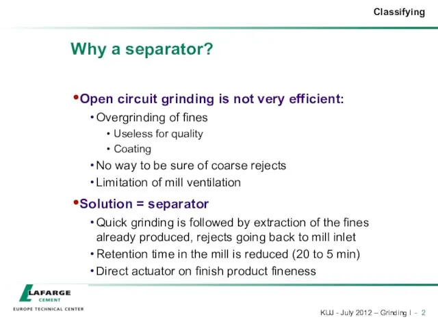
Why a separator?
Open circuit grinding is not very efficient:
Overgrinding of fines
Useless
Why a separator?
Open circuit grinding is not very efficient:
Overgrinding of fines
Useless
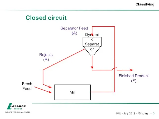
Closed circuit
Closed circuit
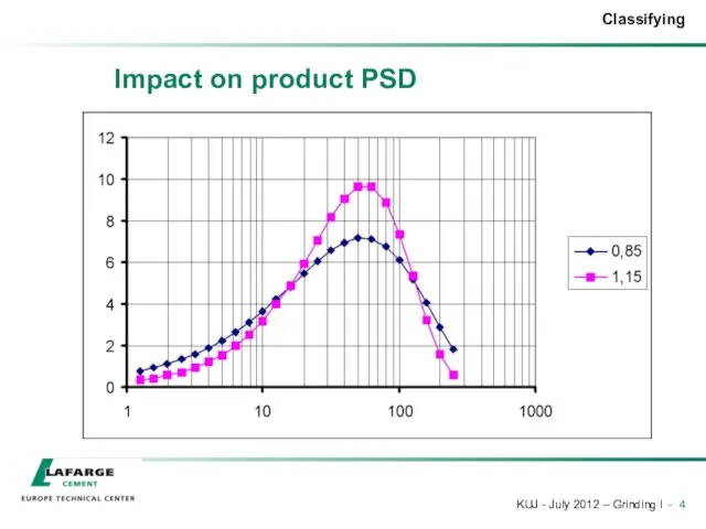
Impact on product PSD
Impact on product PSD
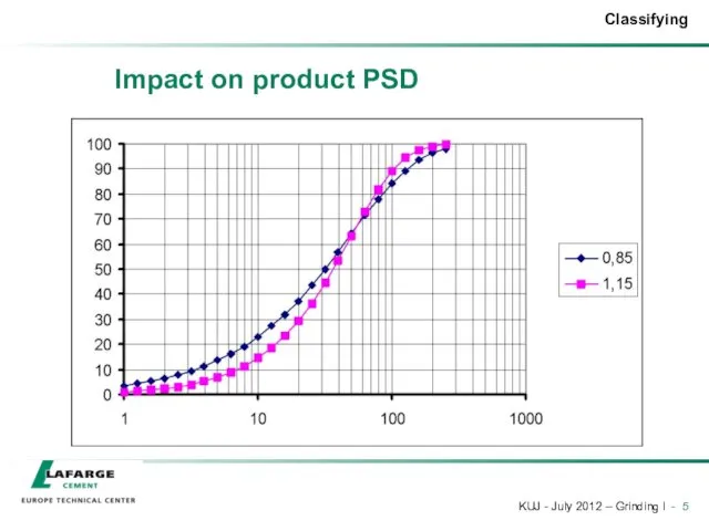
Impact on product PSD
Impact on product PSD
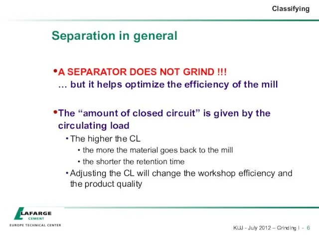
Separation in general
A SEPARATOR DOES NOT GRIND !!!
… but it helps
Separation in general
A SEPARATOR DOES NOT GRIND !!! … but it helps
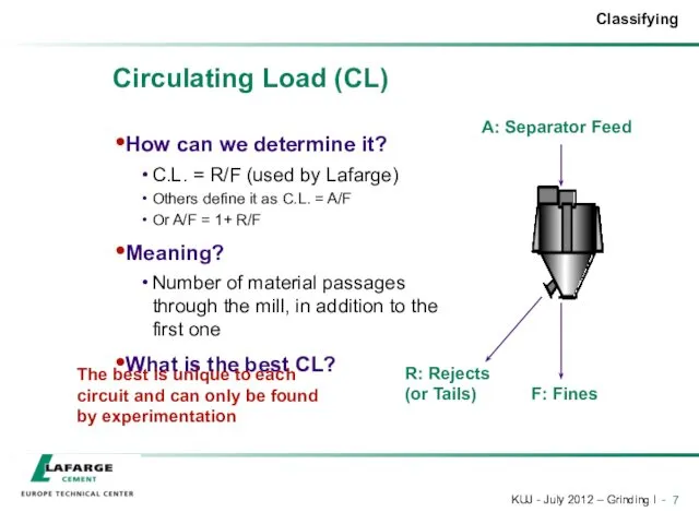
Circulating Load (CL)
How can we determine it?
C.L. = R/F (used by
Circulating Load (CL)
How can we determine it?
C.L. = R/F (used by
Separation efficiency
How do we assess the efficiency of separation?
The tool is
Separation efficiency
How do we assess the efficiency of separation?
The tool is
Separation efficiency
What do we expect of a separator?
Feed PSD
Ideal separation
Real separation
Tromp
Separation efficiency
What do we expect of a separator?
Feed PSD
Ideal separation
Real separation
Tromp
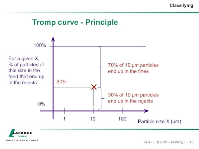
Tromp curve - Principle
Particle size X (µm)
For a given X, %
Tromp curve - Principle
Particle size X (µm)
For a given X, %
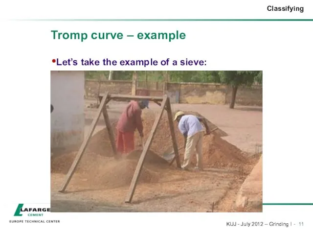
Tromp curve – example
Let’s take the example of a sieve:
Tromp curve – example
Let’s take the example of a sieve:
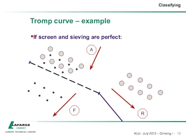
Tromp curve – example
If screen and sieving are perfect:
A
F
R
Tromp curve – example
If screen and sieving are perfect:
A
F
R
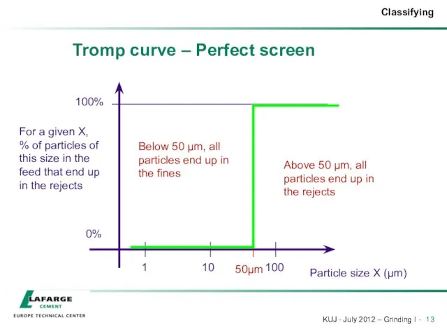
Tromp curve – Perfect screen
50µm
Above 50 µm, all particles end up
Tromp curve – Perfect screen
50µm
Above 50 µm, all particles end up
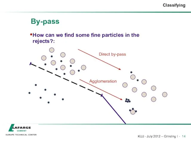
By-pass
How can we find some fine particles in the rejects?:
By-pass
How can we find some fine particles in the rejects?:
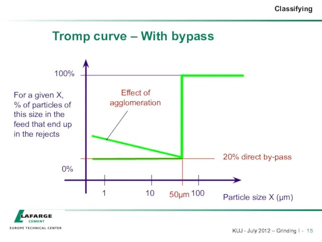
Tromp curve – With bypass
50µm
20% direct by-pass
Tromp curve – With bypass
50µm
20% direct by-pass
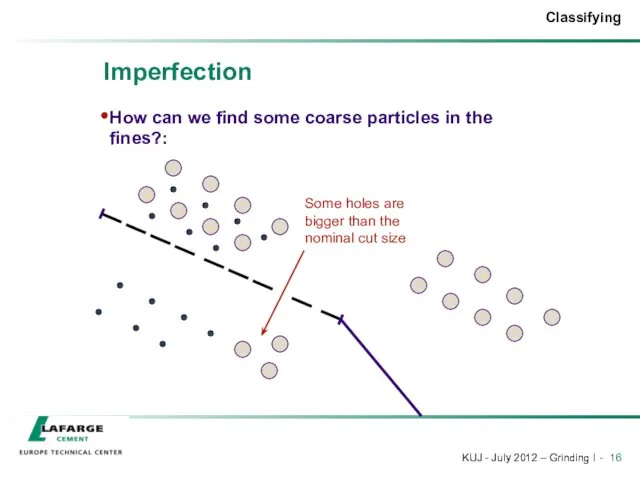
Imperfection
How can we find some coarse particles in the fines?:
Imperfection
How can we find some coarse particles in the fines?:
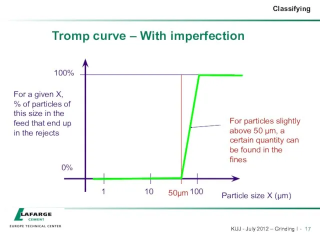
Tromp curve – With imperfection
50µm
For particles slightly above 50 µm, a
Tromp curve – With imperfection
50µm
For particles slightly above 50 µm, a
Tromp curve – General case
By Pass: Lowest percentage of feed that
Tromp curve – General case
By Pass: Lowest percentage of feed that
Tromp curve - Interpretation
By-pass
Should be as low as possible
Directly linked to
Tromp curve - Interpretation
By-pass
Should be as low as possible
Directly linked to
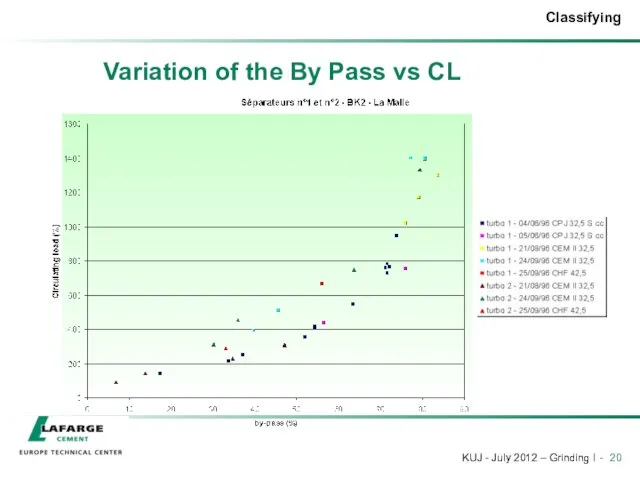
Variation of the By Pass vs CL
Variation of the By Pass vs CL
Tromp curve - Interpretation
Acuity limit
Mainly depends on the fineness of final
Tromp curve - Interpretation
Acuity limit
Mainly depends on the fineness of final
Tromp curve
1st generation (Heydt)
2nd generation (Wedag)
3rd generation (Osepa)
Tromp curve
1st generation (Heydt)
2nd generation (Wedag)
3rd generation (Osepa)
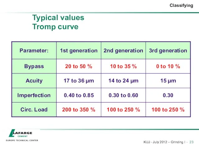
Typical values
Tromp curve
Typical values
Tromp curve
Building a Tromp curve
Mass balance
Knowledge of a physical property of 3
Building a Tromp curve
Mass balance
Knowledge of a physical property of 3
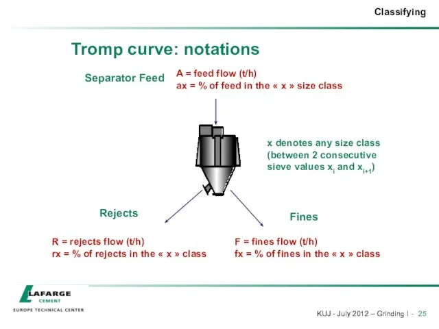
Tromp curve: notations
Separator Feed
Fines
Rejects
A = feed flow (t/h)
ax = % of
Tromp curve: notations
Separator Feed
Fines
Rejects
A = feed flow (t/h)
ax = % of
Tromp curves – R/A calculation
Global mass balance:
A = R + F
Tromp curves – R/A calculation
Global mass balance:
A = R + F
3 point junction (ABC formula)
Example:
Feed 3000 Blaine
Rejects 2000 Blaine
Product 3800
3 point junction (ABC formula)
Example:
Feed 3000 Blaine
Rejects 2000 Blaine
Product 3800
3 point junction (ABC formula)
Example:
Feed 3000 Blaine
Rejects 2000 Blaine
Product 3800
3 point junction (ABC formula)
Example:
Feed 3000 Blaine
Rejects 2000 Blaine
Product 3800
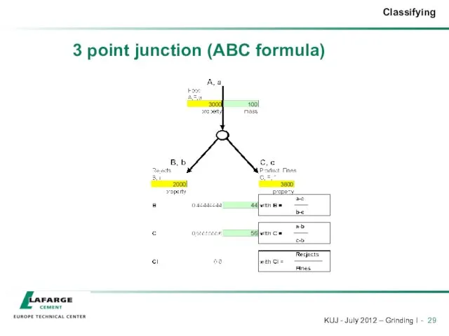
3 point junction (ABC formula)
3 point junction (ABC formula)
Tromp curves – R/A calculation
Interpretation:
Using the laser PSD for separator feed,
Tromp curves – R/A calculation
Interpretation:
Using the laser PSD for separator feed,
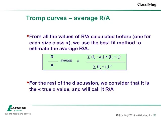
Tromp curves – average R/A
From all the values of R/A calculated
Tromp curves – average R/A
From all the values of R/A calculated
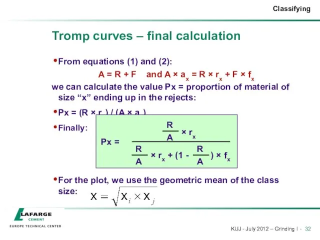
Tromp curves – final calculation
From equations (1) and (2):
A = R
Tromp curves – final calculation
From equations (1) and (2):
A = R
 Викторина Жизнь и творчество С.А. Есенина
 Характеристика методов диагностики заболевания и контроля за эффективностью и безопасностью применения лекарственных средств
 Модульная технология обучения на уроках биологии
 ФГОС - презентация
 Brawlhalla и её движок
 Плата сбора данных ЛА 2М3
 Анализаторы, их строение и функции
 Оформление сертификатов
 Психологические механизмы волевой регуляции. В. А. Иванников
 Инструкция по выгодной продаже недвижимости от АН Держава
 Будущее робототехники. История появления и развития, предназначение и перспективы робототехники
 кл Безопасность в социальных сетях
 формирование ключевых компетенций учащихся на уроках химии как средство реализации личностно-ориентированного подхода в образовании.
 Аудит кредитных операций
 Образцовый Театр Моды Стиль, коллекция Овощной микс
 Презентация. МАСТЕР- КЛАСС.Чудеса солёного теста.
 Возрастные особенности шестиклассников
 презентация на тему: Совершенствование системы физкультурно-оздоровительной работы...
 Прием в 1 класс
 Презентация по ПДД
 Флуктуации амплитуды и частоты в автогенераторах СВЧ
 Великобритания
 Искусство Японии
 Электрические нагрузки промышленных предприятий. Номинальные режимы работы ЭП
 Жизнь птиц и зверей
 Эвенки – народы Байкала
 Презентация Окислительные свойства азотной кислоты
 Игра в черное и белое