- Geodetic control network. (Lecture 4)

Содержание
- 2. Outline Computations on the ellipsoid Ellipsoidal curves (normal sections, curve of alignment, the geodesic); The computation
- 3. The ellipsoidal curves The normal section and the reverse normal section The curve of alignment The
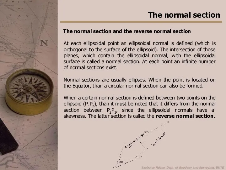
- 4. The normal section The normal section and the reverse normal section At each ellipsoidal point an
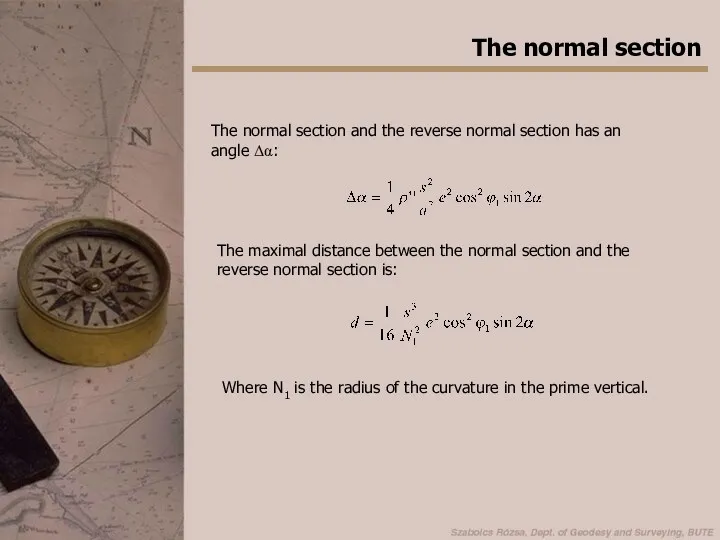
- 5. The normal section The normal section and the reverse normal section has an angle Δα: The
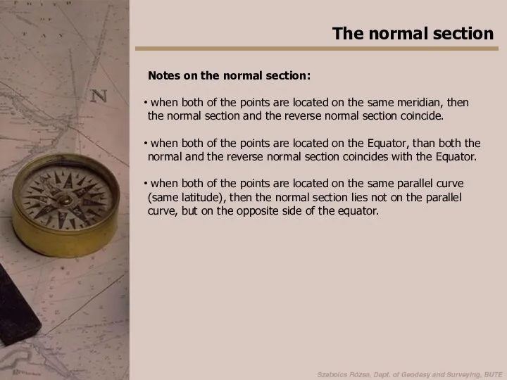
- 6. The normal section Notes on the normal section: when both of the points are located on
- 7. When we want measure the angles of a triangle and connect the nodes of the triangle
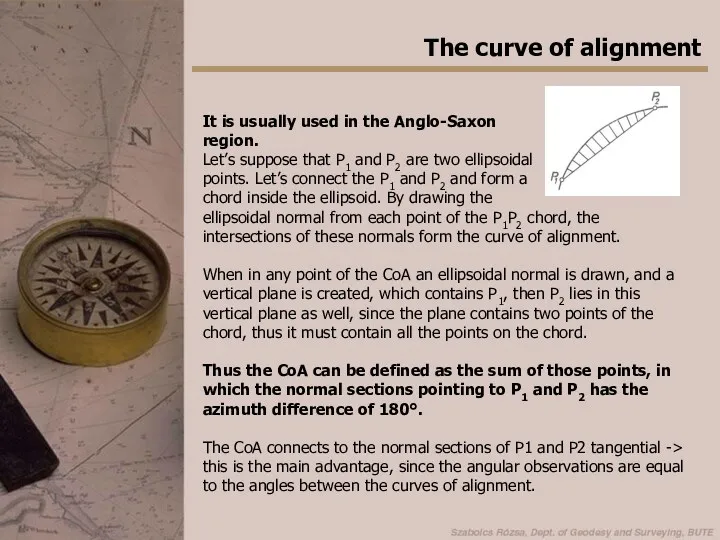
- 8. The curve of alignment It is usually used in the Anglo-Saxon region. Let’s suppose that P1
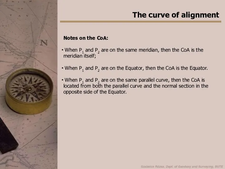
- 9. The curve of alignment Notes on the CoA: When P1 and P2 are on the same
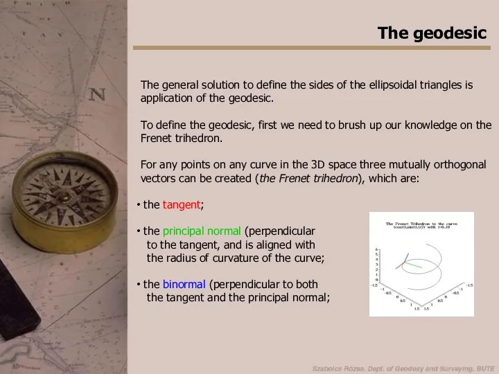
- 10. The geodesic The general solution to define the sides of the ellipsoidal triangles is application of
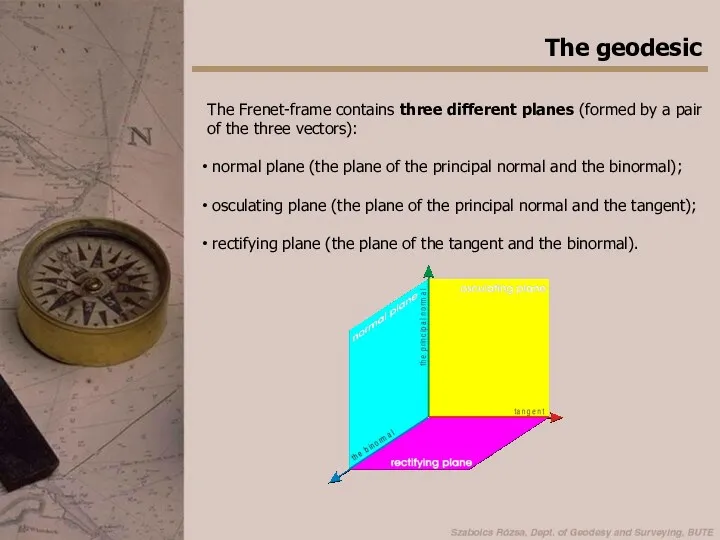
- 11. The geodesic The Frenet-frame contains three different planes (formed by a pair of the three vectors):
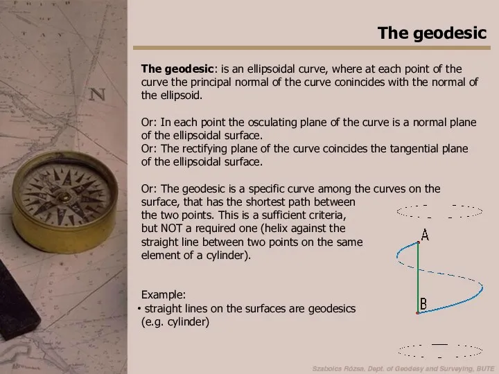
- 12. The geodesic The geodesic: is an ellipsoidal curve, where at each point of the curve the
- 13. Graphical derivation of geodesic on the ell.
- 14. Properties of the geodesic
- 15. The geodesic on surfaces of rotation On surfaces of rotation the following equation can be derived
- 16. The solution of ellipsoidal triangles The ellipsoid is usually approximated by a sphere. When the study
- 17. The excess angle of the ellipsoidal triangle Ellipsoidal triangles are approximated by sperical tirangles. The spherical
- 18. The excess angle of the ellipsoidal triangle The excess angle: In case of large triangles (bigger
- 19. The Legendre method The ellipsodal triangles are approximated by spherical triangles (Gauss-theorem) that has the same
- 20. The Legendre method When the spherical (ellipsoidal) triangle is not small enough, then Note: the difference
- 21. The Soldner method Additive constants
- 22. The computation of coordinates on the ell. 1st and 2nd fundamental task solving polar ellipsoidal triangles
- 23. The computation of coordinates on the ell. Various solution depending on the distance: up to 200
- 24. 1st fundamental task Legendre’s polynomial method Known P1 (ϕ1,λ1) and α1,2, then the ϕ2,λ2 coordinates and
- 25. Legendre’s polynomial method The differential equation system of the geodesic
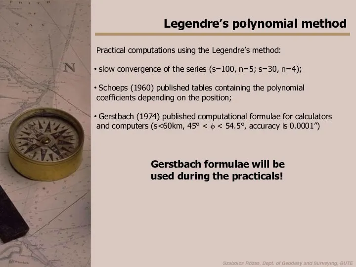
- 26. Legendre’s polynomial method Practical computations using the Legendre’s method: slow convergence of the series (s=100, n=5;
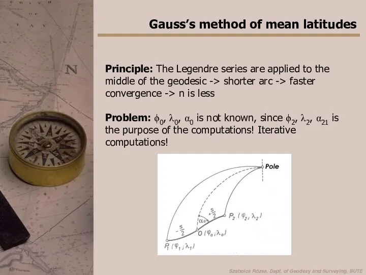
- 27. Gauss’s method of mean latitudes Principle: The Legendre series are applied to the middle of the
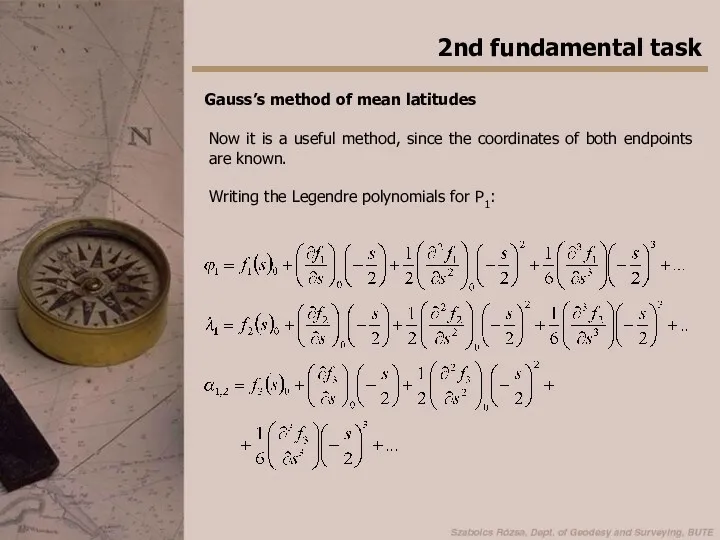
- 28. 2nd fundamental task Gauss’s method of mean latitudes Now it is a useful method, since the
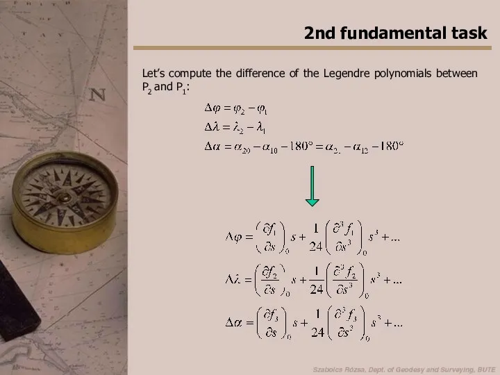
- 29. Writing the Legendre polynomials for P2: 2nd fundamental task Where:
- 30. 2nd fundamental task Let’s compute the difference of the Legendre polynomials between P2 and P1:
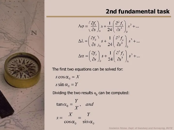
- 31. 2nd fundamental task The first two equations can be solved for: Dividing the two results α0
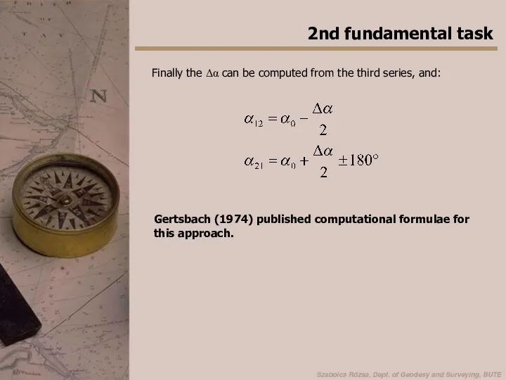
- 32. 2nd fundamental task Finally the Δα can be computed from the third series, and: Gertsbach (1974)
- 34. Скачать презентацию
Outline
Computations on the ellipsoid
Ellipsoidal curves (normal sections, curve of alignment,
Outline
Computations on the ellipsoid
Ellipsoidal curves (normal sections, curve of alignment,
The ellipsoidal curves
The normal section and the reverse normal section
The curve
The ellipsoidal curves
The normal section and the reverse normal section
The curve
The normal section
The normal section and the reverse normal section
At each
The normal section
The normal section and the reverse normal section
At each
The normal section
The normal section and the reverse normal section has
The normal section
The normal section and the reverse normal section has
The normal section
Notes on the normal section:
when both of the
The normal section
Notes on the normal section:
when both of the
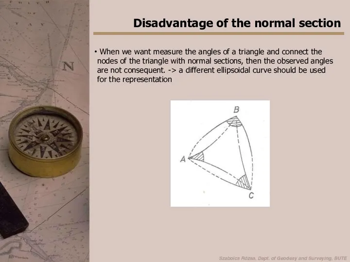
When we want measure the angles of a triangle and
When we want measure the angles of a triangle and
The curve of alignment
It is usually used in the Anglo-Saxon
region.
The curve of alignment
It is usually used in the Anglo-Saxon
region.
The curve of alignment
Notes on the CoA:
When P1 and P2
The curve of alignment
Notes on the CoA:
When P1 and P2
The geodesic
The general solution to define the sides of the ellipsoidal
The geodesic
The general solution to define the sides of the ellipsoidal
The geodesic
The Frenet-frame contains three different planes (formed by a pair
The geodesic
The Frenet-frame contains three different planes (formed by a pair
The geodesic
The geodesic: is an ellipsoidal curve, where at each point
The geodesic
The geodesic: is an ellipsoidal curve, where at each point
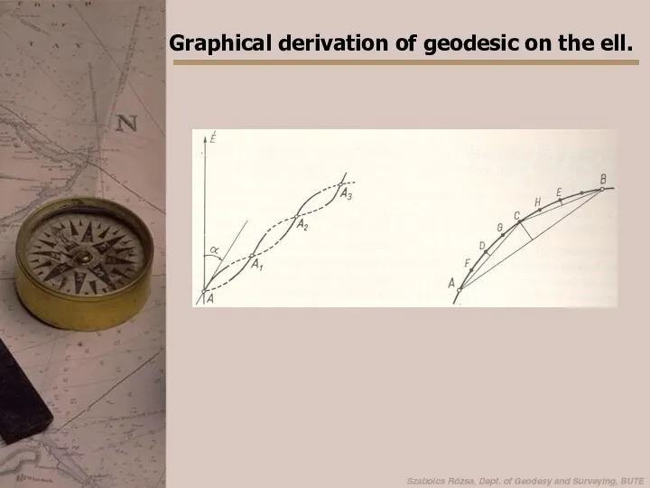
Graphical derivation of geodesic on the ell.
Graphical derivation of geodesic on the ell.
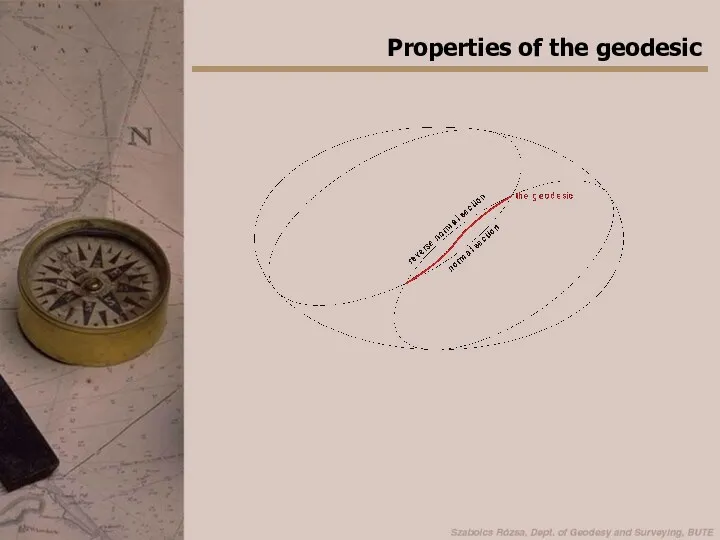
Properties of the geodesic
Properties of the geodesic
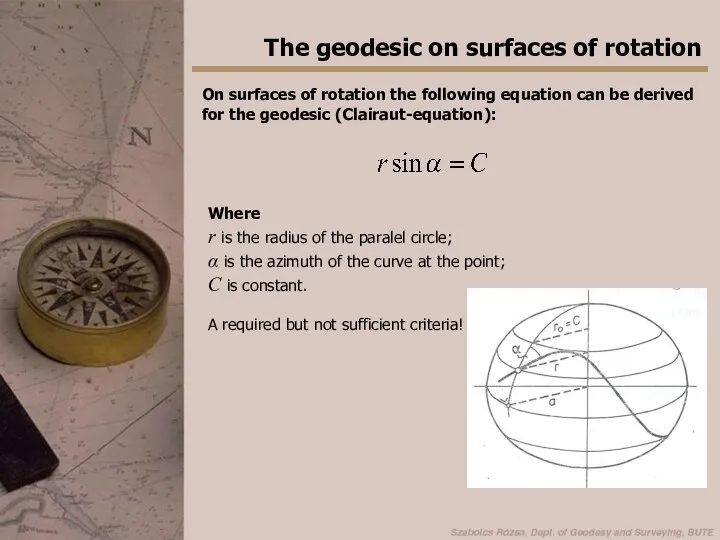
The geodesic on surfaces of rotation
On surfaces of rotation the following
The geodesic on surfaces of rotation
On surfaces of rotation the following
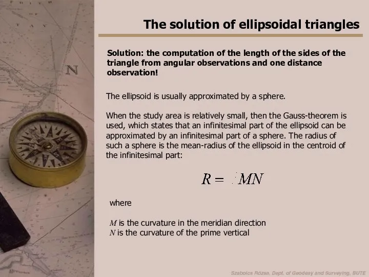
The solution of ellipsoidal triangles
The ellipsoid is usually approximated by a
The solution of ellipsoidal triangles
The ellipsoid is usually approximated by a
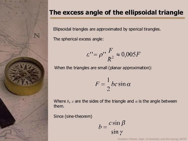
The excess angle of the ellipsoidal triangle
Ellipsoidal triangles are approximated by
The excess angle of the ellipsoidal triangle
Ellipsoidal triangles are approximated by
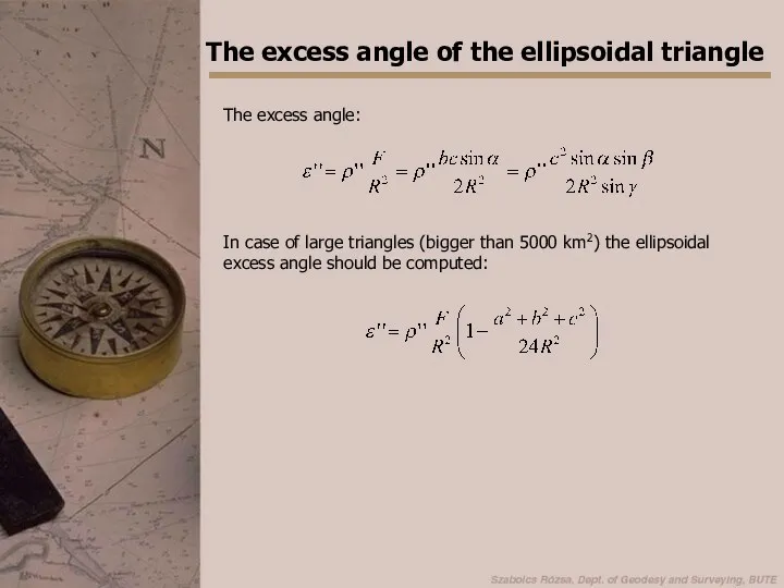
The excess angle of the ellipsoidal triangle
The excess angle:
In case of
The excess angle of the ellipsoidal triangle
The excess angle:
In case of
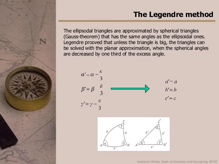
The Legendre method
The ellipsodal triangles are approximated by spherical triangles (Gauss-theorem)
The Legendre method
The ellipsodal triangles are approximated by spherical triangles (Gauss-theorem)
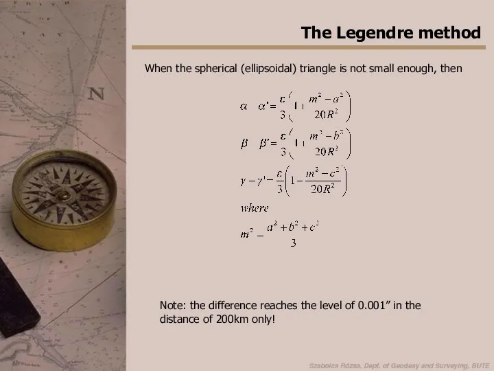
The Legendre method
When the spherical (ellipsoidal) triangle is not small enough,
The Legendre method
When the spherical (ellipsoidal) triangle is not small enough,
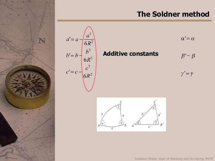
The Soldner method
Additive constants
The Soldner method
Additive constants
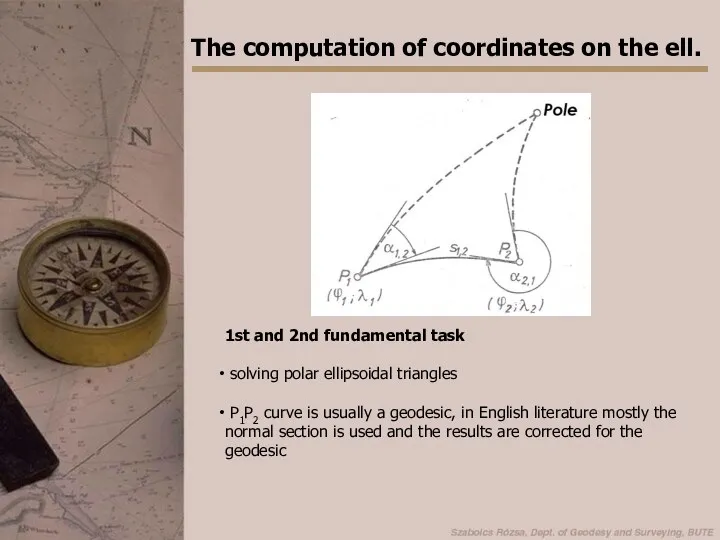
The computation of coordinates on the ell.
1st and 2nd fundamental task
The computation of coordinates on the ell.
1st and 2nd fundamental task
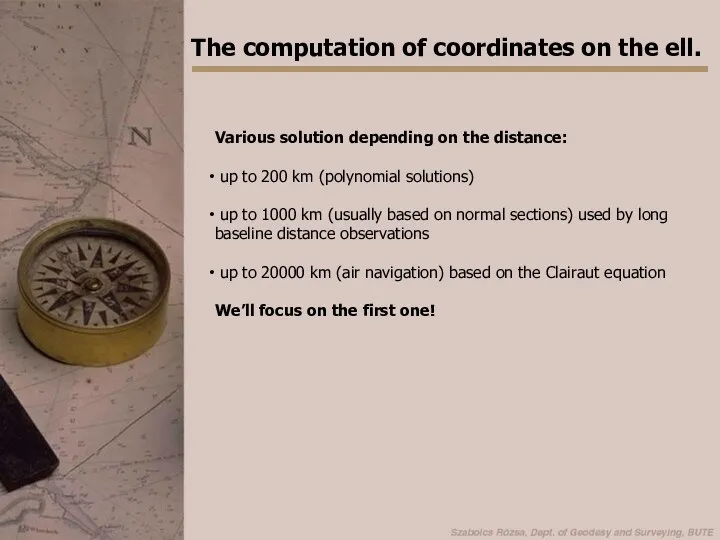
The computation of coordinates on the ell.
Various solution depending on the
The computation of coordinates on the ell.
Various solution depending on the
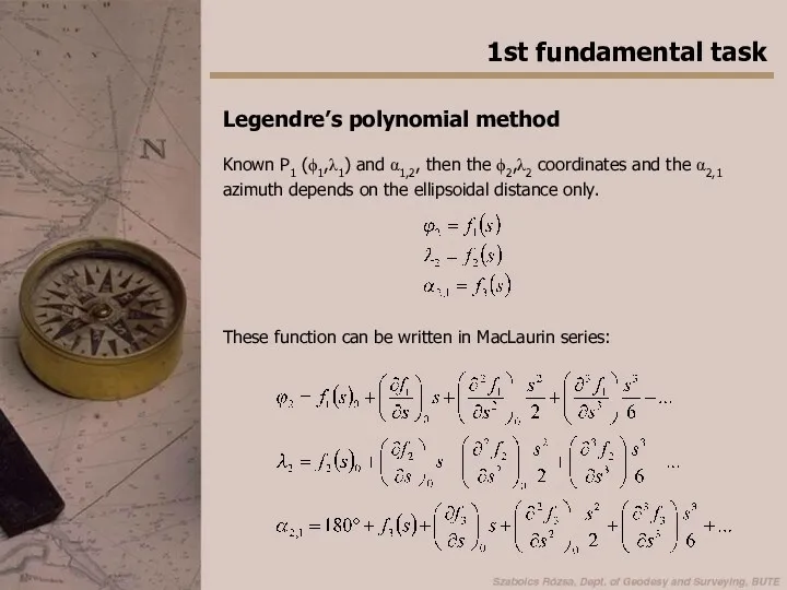
1st fundamental task
Legendre’s polynomial method
Known P1 (ϕ1,λ1) and α1,2, then the
1st fundamental task
Legendre’s polynomial method
Known P1 (ϕ1,λ1) and α1,2, then the
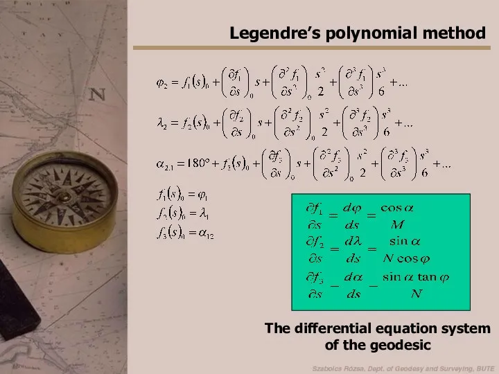
Legendre’s polynomial method
The differential equation system
of the geodesic
Legendre’s polynomial method
The differential equation system
of the geodesic
Legendre’s polynomial method
Practical computations using the Legendre’s method:
slow convergence of
Legendre’s polynomial method
Practical computations using the Legendre’s method:
slow convergence of
Gauss’s method of mean latitudes
Principle: The Legendre series are applied to
Gauss’s method of mean latitudes
Principle: The Legendre series are applied to
2nd fundamental task
Gauss’s method of mean latitudes
Now it is a useful
2nd fundamental task
Gauss’s method of mean latitudes
Now it is a useful
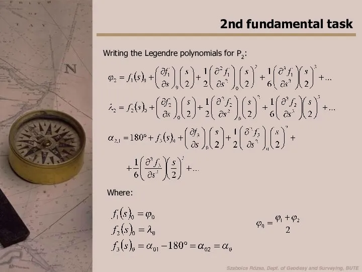
Writing the Legendre polynomials for P2:
2nd fundamental task
Where:
Writing the Legendre polynomials for P2:
2nd fundamental task
Where:
2nd fundamental task
Let’s compute the difference of the Legendre polynomials between
2nd fundamental task
Let’s compute the difference of the Legendre polynomials between
2nd fundamental task
The first two equations can be solved for:
Dividing
2nd fundamental task
The first two equations can be solved for:
Dividing
2nd fundamental task
Finally the Δα can be computed from the third
2nd fundamental task
Finally the Δα can be computed from the third
 Опасный мусор. Правильная утилизация батареек
 Процессы водоподготовки и очистки сточных вод
 Мусор до нуля. Выбери нужный контейнер
 Эколята – дошколята
 Экология. Безопасность. Жизнь
 Третье задание вятгуchallenge. 33 команда
 Кислотные дожди
 Среды жизни планеты Земля
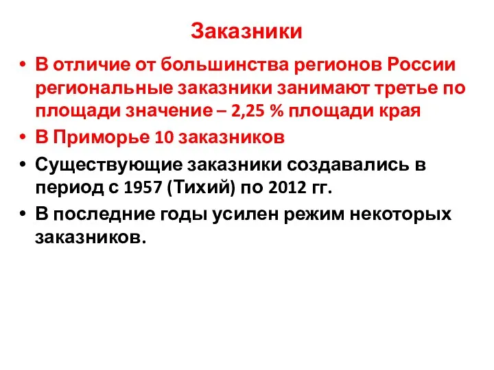 Заказники Приморского края
 Екомаршрут: Карпатський національний природний парк
 Загрязнение атмосферы
 Отчет о проведении краевой экологической акции Зеленая волна
 Социологическое исследование Удовлетворенность качеством и комфортом городской среды
 Глобальные проблемы современности
 Повторное использование бытовых отходов
 Экологические проблемы и её классификация
 Пути решения глобальных проблем
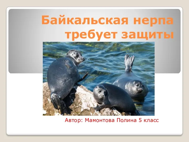 Байкальская нерпа требует защиты. 5 класс
 Environmental issues
 презентация Исследовательская работа Влияние шума на здоровье человека
 Эколого-просветительский проект Природа - наш дом
 Определение показателей химического загрязнения почв
 Биосфера, её структура и функции
 Сторінками червоної книги України
 Рациональное использование и охрана лесов в России
 Аутэкология. Организм және қоршаған орта. Тірі жүйелердің ұйымдасу деңгейі
 I have a dream to make my Region better
 Кліматотвірні чинники. Розподіл сонячної енергії на Землі