- 10 principles of economics

Содержание
- 2. Economy… . . . The word economy comes from a Greek word for “one who manages
- 3. PRINCIPLES OF ECONOMICS A household and an economy face many decisions: Who will work? What goods
- 4. PRINCIPLES OF ECONOMICS Society and Scarce Resources: The management of society’s resources is important because resources
- 5. Economics Economics is the study of how society manages its scarce resources. The branch of knowledge
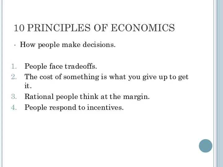
- 6. 10 PRINCIPLES OF ECONOMICS How people make decisions. People face tradeoffs. The cost of something is
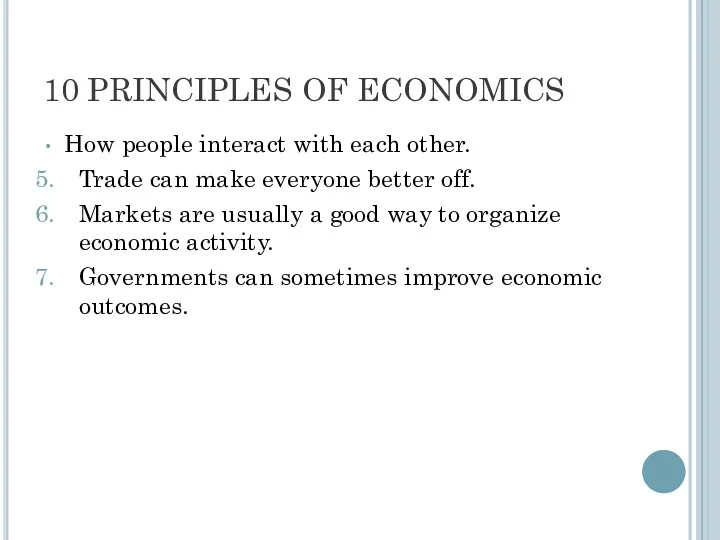
- 7. 10 PRINCIPLES OF ECONOMICS How people interact with each other. Trade can make everyone better off.
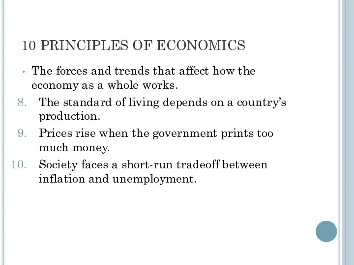
- 8. 10 PRINCIPLES OF ECONOMICS The forces and trends that affect how the economy as a whole
- 9. Principle #1: People Face Tradeoffs Trade off is a situation that involves losing one quality or
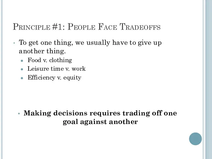
- 10. Principle #1: People Face Tradeoffs To get one thing, we usually have to give up another
- 11. Principle #1: People Face Tradeoffs Efficiency v. Equity Efficiency means society gets the most that it
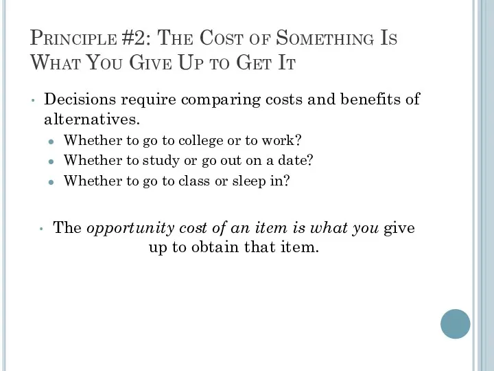
- 12. Principle #2: The Cost of Something Is What You Give Up to Get It Decisions require
- 13. Principle #2: The Cost of Something Is What You Give Up to Get It Cricketing god
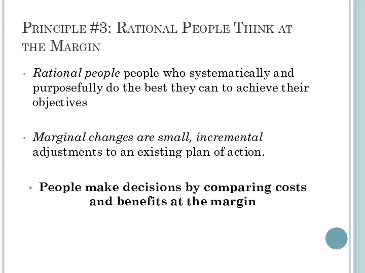
- 14. Principle #3: Rational People Think at the Margin Rational people people who systematically and purposefully do
- 15. Principle #4: People Respond to Incentives Incentives – something that induces a person to act Marginal
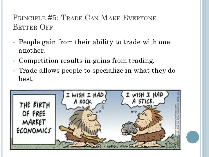
- 16. Principle #5: Trade Can Make Everyone Better Off People gain from their ability to trade with
- 17. Principle #6: Markets Are Usually a Good Way to Organize Economic Activity A market economy is
- 18. Principle #6: Markets Are Usually a Good Way to Organize Economic Activity Adam Smith made the
- 19. Principle #7: Governments Can Sometimes Improve Market Outcomes Market failure occurs when the market fails to
- 20. Principle #7: Governments Can Sometimes Improve Market Outcomes Market failure may be caused by an externality,
- 21. Principle #8: The Standard of Living Depends on a Country’s Production Standard of living may be
- 22. Principle #8: The Standard of Living Depends on a Country’s Production Almost all variations in living
- 23. Principle #9: Prices Rise When the Government Prints Too Much Money Inflation is an increase in
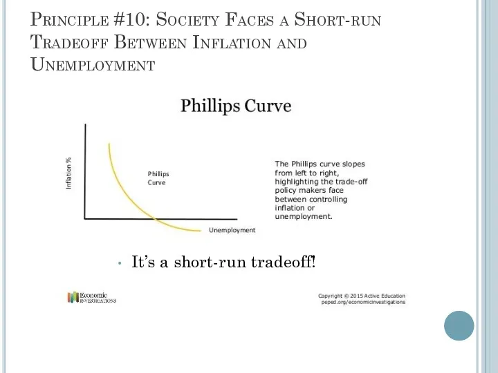
- 24. Principle #10: Society Faces a Short-run Tradeoff Between Inflation and Unemployment It’s a short-run tradeoff!
- 25. Summary When individuals make decisions, they face tradeoffs among alternative goals. The cost of any action
- 26. Summary Trade can be mutually beneficial. Markets are usually a good way of coordinating trade among
- 27. Summary Productivity is the ultimate source of living standards. Money growth is the ultimate source of
- 28. Macroeconomics Introduction to Macroeconomics Zharova Liubov Zharova_l@ua.fm
- 29. Intro individual decision-making Microeconomics examines the behavior of units—business firms and households. Macroeconomics deals with the
- 30. Intro When we study the consumption behaviour or equilibrium of a consumer; the production pattern &
- 31. Intro Microeconomists generally conclude that markets work well. Macroeconomists, however, observe that some important prices often
- 32. Intro Macroeconomists often reflect on the microeconomic principles underlying macroeconomic analysis, or the microeconomic foundations of
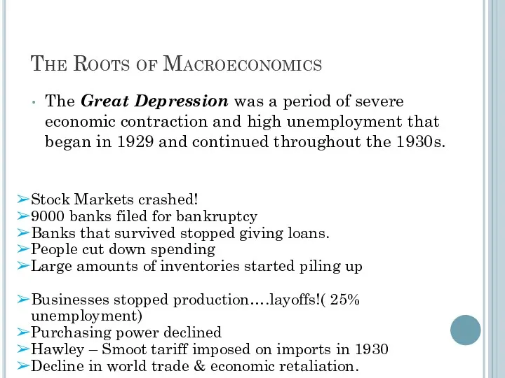
- 33. The Roots of Macroeconomics The Great Depression was a period of severe economic contraction and high
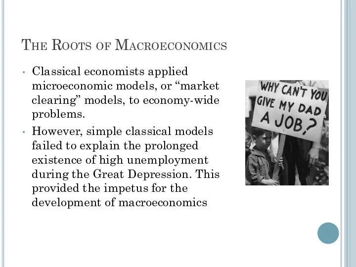
- 34. The Roots of Macroeconomics Classical economists applied microeconomic models, or “market clearing” models, to economy-wide problems.
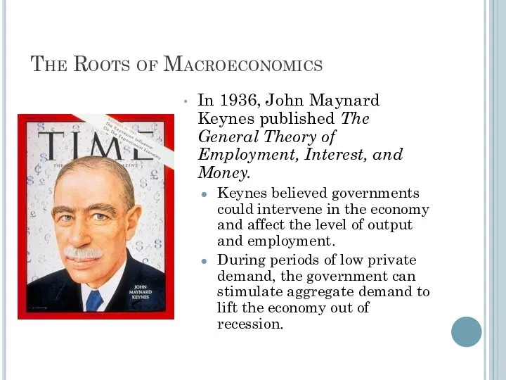
- 35. The Roots of Macroeconomics In 1936, John Maynard Keynes published The General Theory of Employment, Interest,
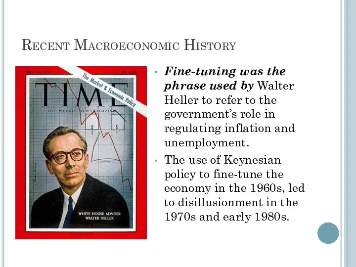
- 36. Recent Macroeconomic History Fine-tuning was the phrase used by Walter Heller to refer to the government’s
- 37. Why to Study Macroeconomics? Macroeconomics is the study of the nation’s economy as a whole. We
- 38. Macroeconomic Concerns Three of the major concerns of macroeconomics are: Inflation Output growth Unemployment
- 39. Inflation and Deflation Inflation is an increase in the overall price level. Hyperinflation is a period
- 40. Inflation
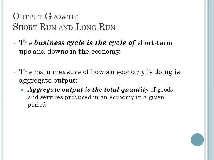
- 41. Output Growth: Short Run and Long Run The business cycle is the cycle of short-term ups
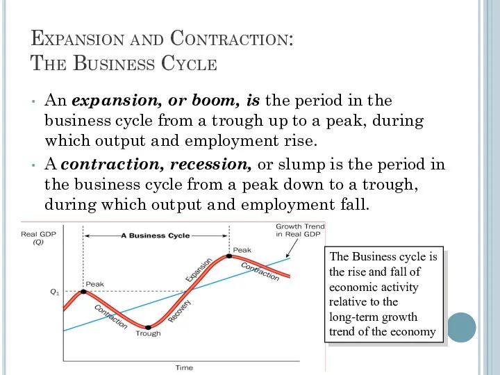
- 42. The Business cycle is the rise and fall of economic activity relative to the long-term growth
- 43. Ups and downs of the Business Cycle Peak: at the peak of the business cycle, Real
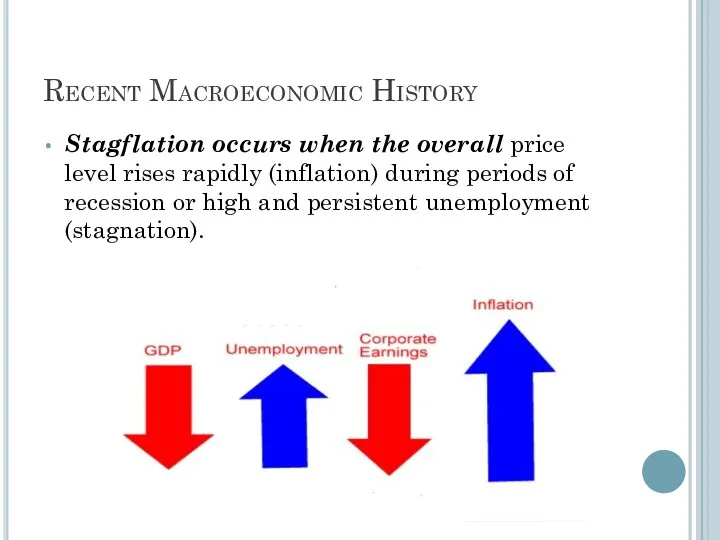
- 44. Recent Macroeconomic History Stagflation occurs when the overall price level rises rapidly (inflation) during periods of
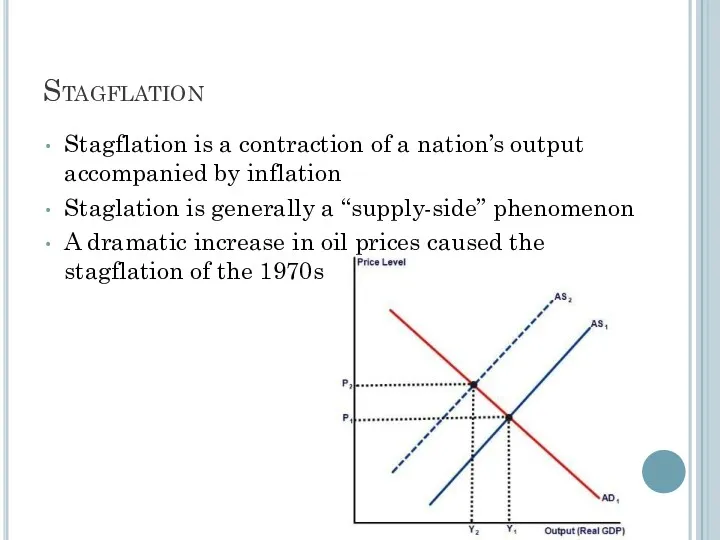
- 45. Stagflation Stagflation is a contraction of a nation’s output accompanied by inflation Staglation is generally a
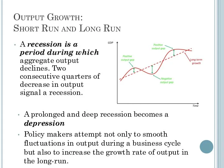
- 46. Output Growth: Short Run and Long Run A recession is a period during which aggregate output
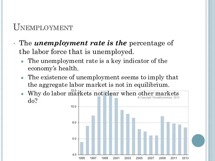
- 47. Unemployment The unemployment rate is the percentage of the labor force that is unemployed. The unemployment
- 48. Unemployment
- 49. Government in the Macroeconomy There are three kinds of policy that the government has used to
- 50. Government in the Macroeconomy Fiscal policy refers to government policies concerning taxes and spending. Monetary policy
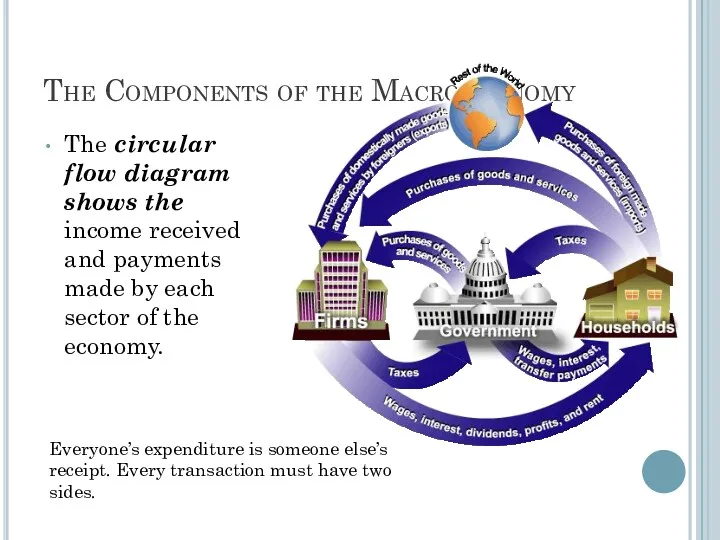
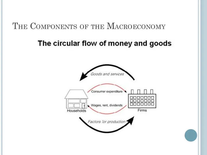
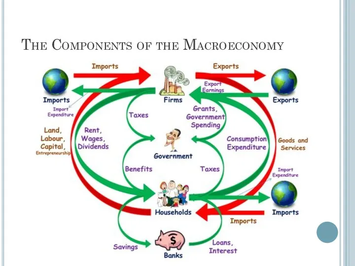
- 51. The Components of the Macroeconomy The circular flow diagram shows the income received and payments made
- 52. The Components of the Macroeconomy
- 53. The Components of the Macroeconomy
- 54. The Components of the Macroeconomy Transfer payments are payments made by the government to people who
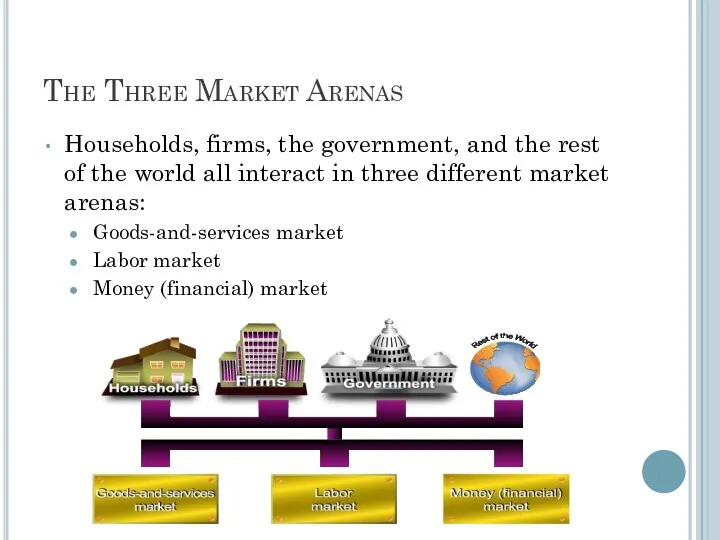
- 55. The Three Market Arenas Households, firms, the government, and the rest of the world all interact
- 56. The Three Market Arenas Households and the government purchase goods and services (demand) from firms in
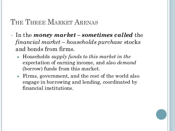
- 57. The Three Market Arenas In the money market – sometimes called the financial market – households
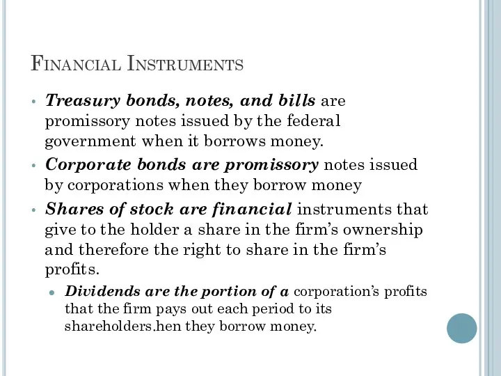
- 58. Financial Instruments Treasury bonds, notes, and bills are promissory notes issued by the federal government when
- 59. The Methodology of Macroeconomics Connections to microeconomics: Macroeconomic behavior is the sum of all the microeconomic
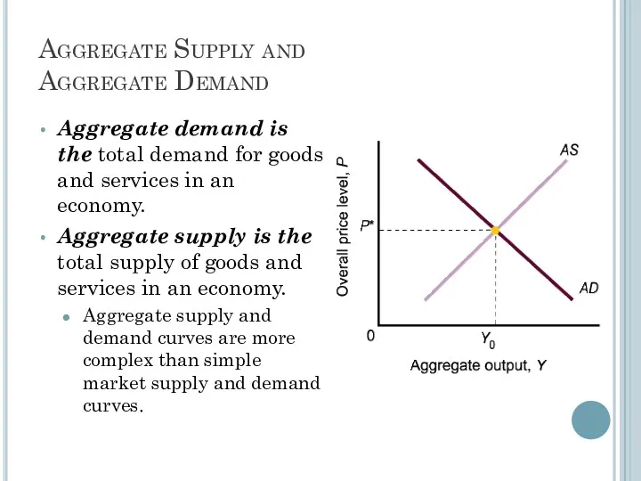
- 60. Aggregate Supply and Aggregate Demand Aggregate demand is the total demand for goods and services in
- 61. Expansion and Contraction: The Business Cycle An expansion, or boom, is the period in the business
- 62. Review Terms and Concepts aggregate behavior aggregate demand aggregate output aggregate supply business cycle circular flow
- 63. Macroeconomics The Measurement and Structure of the National Economy Zharova Liubov Zharova_l@ua.fm
- 64. Outline National Income Accounting: The Measurement of Production, Income, and Expenditure Gross Domestic Product Saving and
- 65. National Income Accounting The national income accounts is an accounting framework used in measuring current economic
- 66. National Income Accounting Business example shows that all three approaches are equal Important concept in product
- 67. National Income Accounting Why are the three approaches equivalent? They must be, by definition Any output
- 68. National Income Accounting Some of the metrics calculated by using national income accounting include Gross Domestic
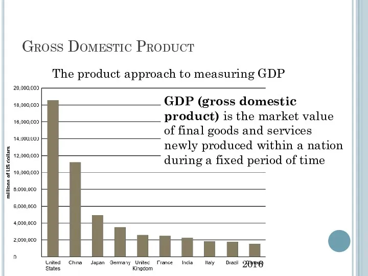
- 69. Gross Domestic Product The product approach to measuring GDP GDP (gross domestic product) is the market
- 70. Gross Domestic Product Market value: allows adding together unlike items by valuing them at their market
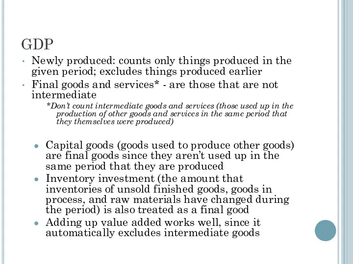
- 72. GDP Newly produced: counts only things produced in the given period; excludes things produced earlier Final
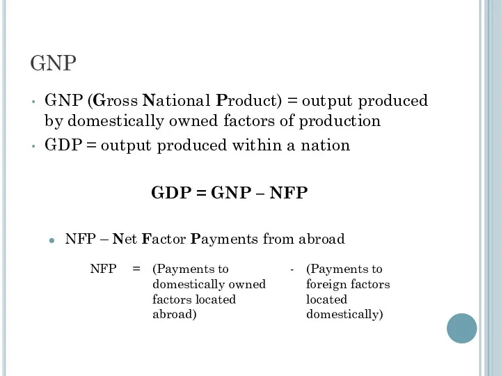
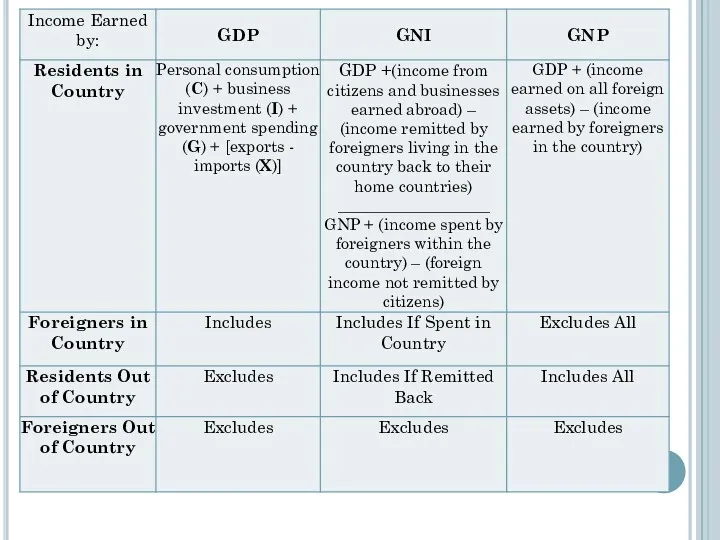
- 73. GNP GNP (Gross National Product) = output produced by domestically owned factors of production GDP =
- 74. GNP Example: Engineering revenues for a road built by a U.S. company in Saudi Arabia is
- 75. Example If a Japanese multinational produces cars in the UK, this production will be counted towards
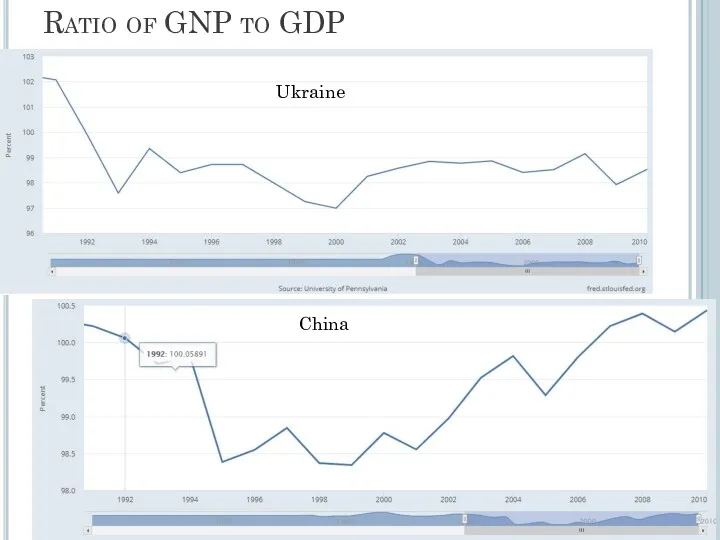
- 76. Ratio of GNP to GDP Ukraine China
- 77. GNI GNI (Gross National Income) – measures income received by a country both domestically and from
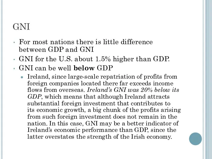
- 78. GNI For most nations there is little difference between GDP and GNI GNI for the U.S.
- 79. To convert a nation’s GDP to GNI Three terms need to be added to the former:
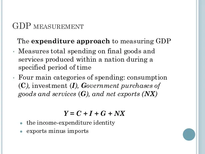
- 82. GDP measurement The expenditure approach to measuring GDP Measures total spending on final goods and services
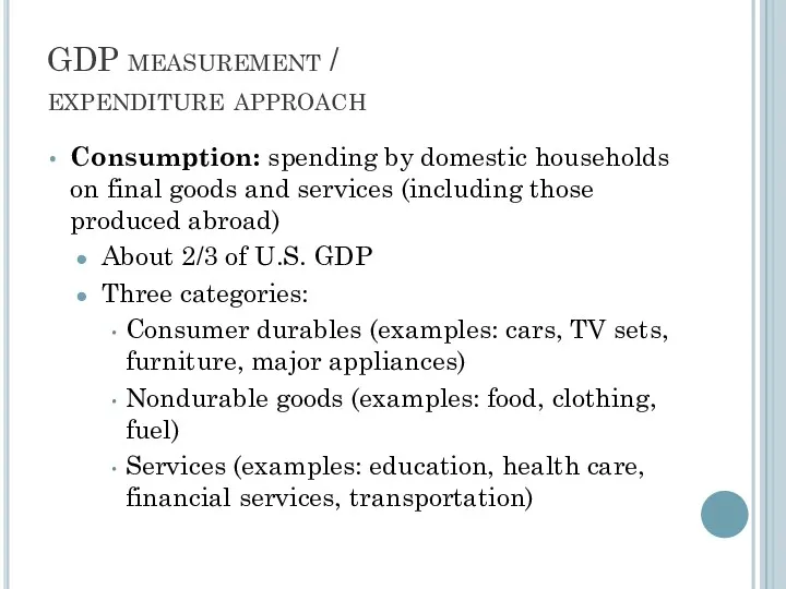
- 83. GDP measurement / expenditure approach Consumption: spending by domestic households on final goods and services (including
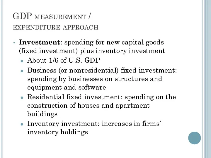
- 84. GDP measurement / expenditure approach Investment: spending for new capital goods (fixed investment) plus inventory investment
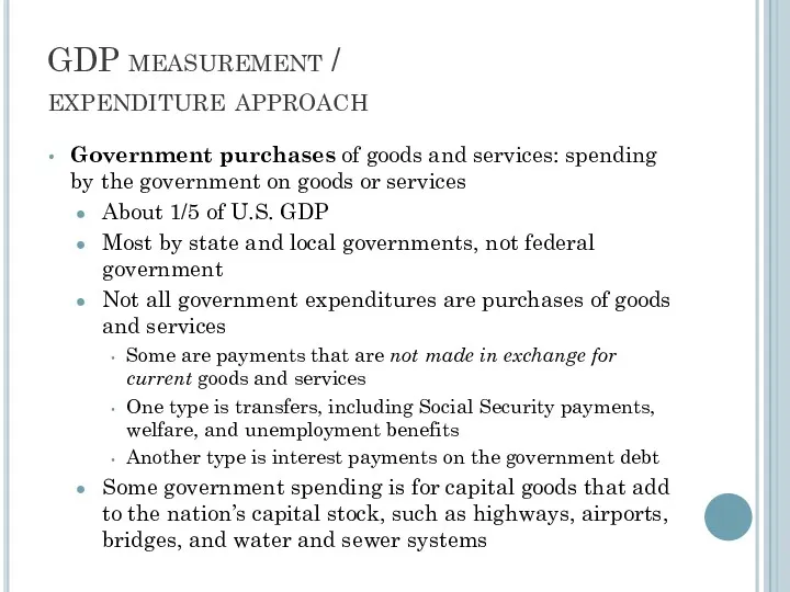
- 85. GDP measurement / expenditure approach Government purchases of goods and services: spending by the government on
- 86. GDP measurement / expenditure approach Net exports: exports minus imports Exports: goods produced in the country
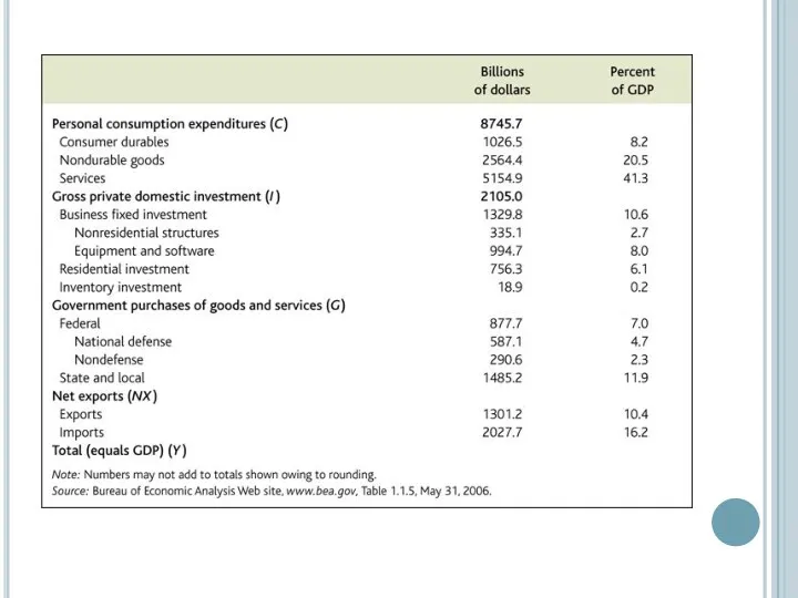
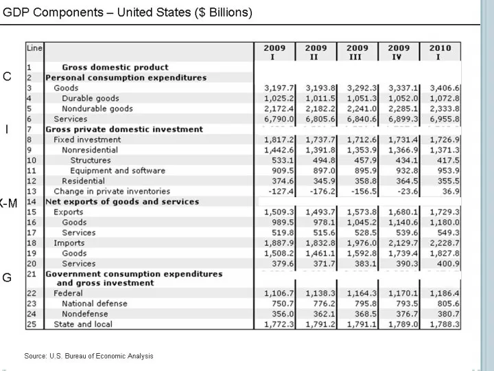
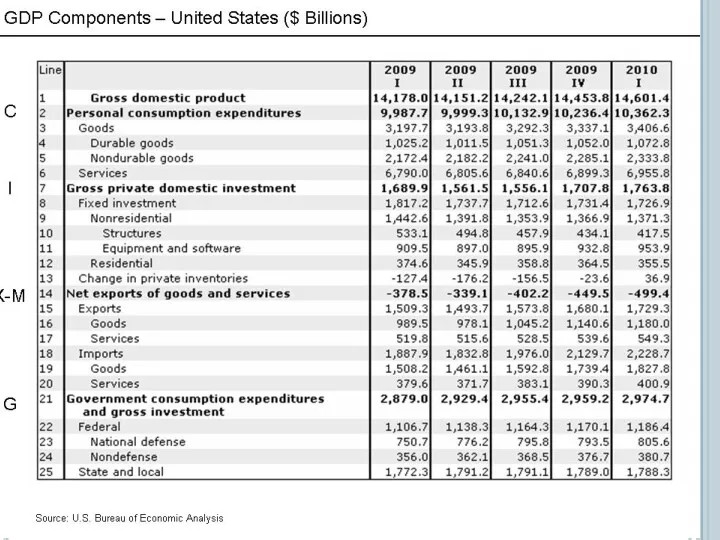
- 87. Expenditure Approach to Measuring GDP (United States)
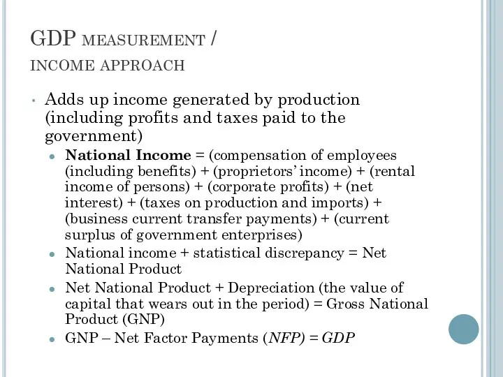
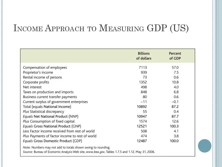
- 88. GDP measurement / income approach Adds up income generated by production (including profits and taxes paid
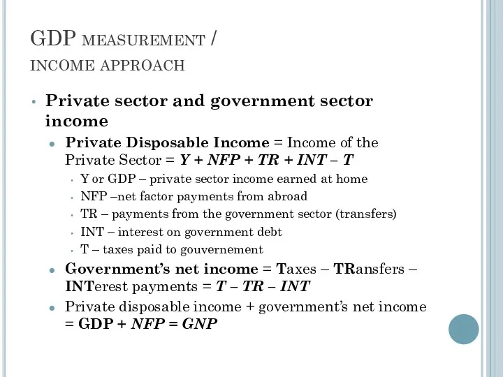
- 89. GDP measurement / income approach Private sector and government sector income Private Disposable Income = Income
- 90. Income Approach to Measuring GDP (US)
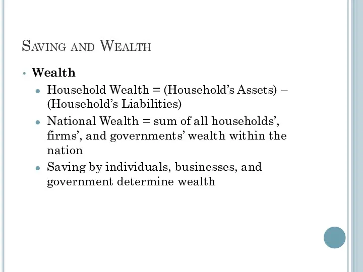
- 91. Saving and Wealth Wealth Household Wealth = (Household’s Assets) – (Household’s Liabilities) National Wealth = sum
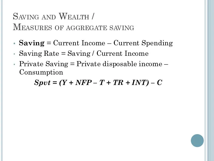
- 92. Saving and Wealth / Measures of aggregate saving Saving = Current Income – Current Spending Saving
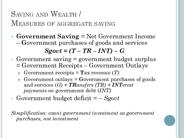
- 93. Saving and Wealth / Measures of aggregate saving Government Saving = Net Government Income – Government
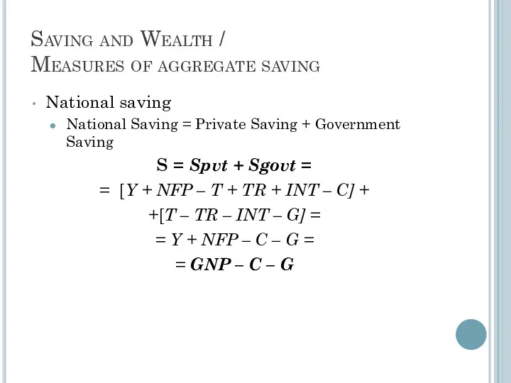
- 94. Saving and Wealth / Measures of aggregate saving National saving National Saving = Private Saving +
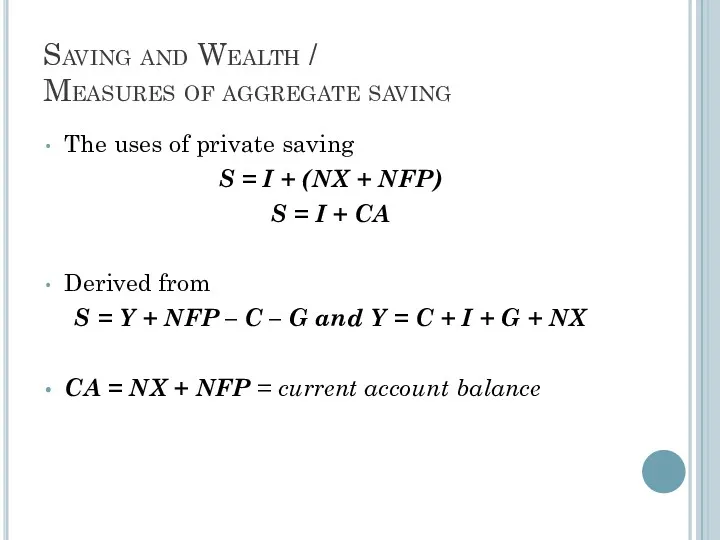
- 95. Saving and Wealth / Measures of aggregate saving The uses of private saving S = I
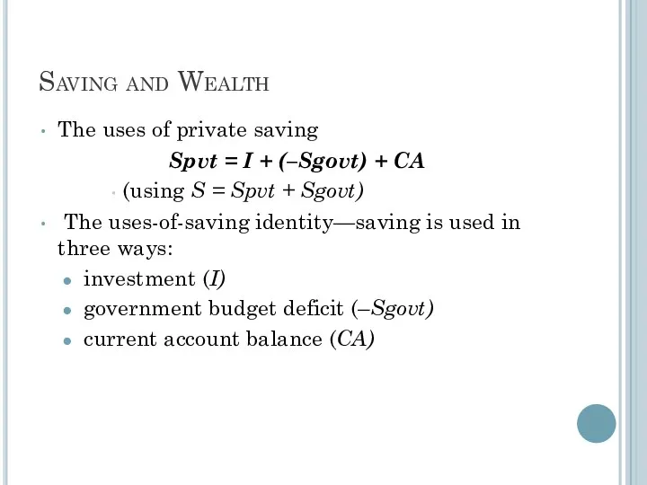
- 96. Saving and Wealth The uses of private saving Spvt = I + (–Sgovt) + CA (using
- 97. Saving and Wealth / Relating saving and wealth Stocks and flows Flow variables: measured per unit
- 98. Saving and Wealth / Relating saving and wealth National wealth: domestic physical assets + net foreign
- 99. Saving and Wealth / Relating saving and wealth National wealth: domestic physical assets + net foreign
- 100. Measures of the Aggregate Savings
- 101. Real GDP, Price Indexes, and Inflation Real GDP Nominal variables are those in dollar terms Problem:
- 102. Computers & Bicycles
- 103. Computers & Bicycles
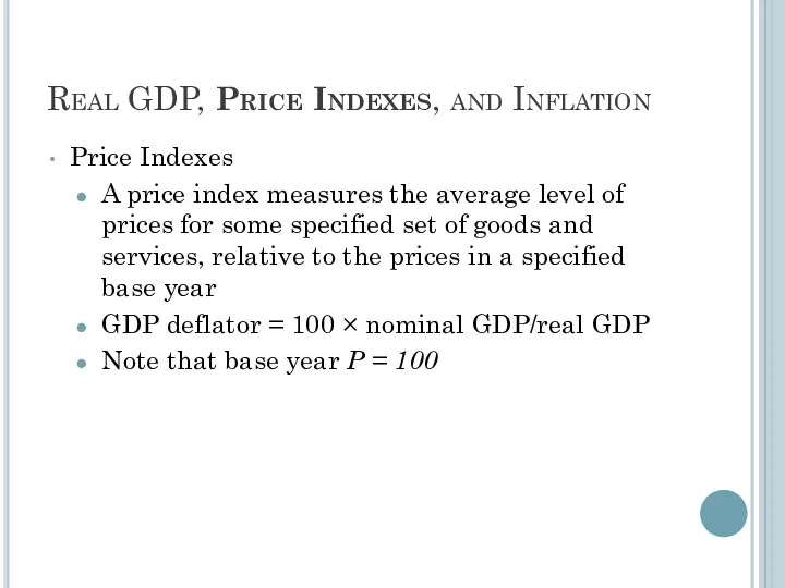
- 104. Real GDP, Price Indexes, and Inflation Price Indexes A price index measures the average level of
- 105. Real GDP, Price Indexes, and Inflation Price Indexes Consumer Price Index (CPI) Price index is a
- 106. Real GDP, Price Indexes, and Inflation Price Indexes GDP Choice of expenditure base period matters for
- 107. Real GDP, Price Indexes, and Inflation Inflation Calculate inflation rate: inflation rate for the GDP deflator
- 108. Real GDP, Price Indexes, and Inflation Price Indexes Does CPI inflation overstate increases in the cost
- 109. Real GDP, Price Indexes, and Inflation Price Indexes Does CPI inflation overstate increases in the cost
- 110. Real GDP, Price Indexes, and Inflation Does CPI inflation overstate increases in the cost of living?
- 111. Interest rate Real vs. nominal interest rates Interest rate: a rate of return promised by a
- 112. Gross National Product (GNP) Gross Domestic Product (GDP) Net National Product (NNP) Net National Income (NNI)
- 113. The balance of payments, also known as balance of international payments of a country is the
- 114. Producer Price Index (PPI) measures the average changes in prices received by domestic producers for their
- 115. Macroeconomics The Measurement and Structure of the National Economy Zharova Liubov Zharova_l@ua.fm
- 117. “It isn’t a case of more globalization or less, but of a different and less predictable
- 118. What Is Globalization Globalization is defined as a process that, based on international strategies, aims to
- 119. basic aspects of globalization In 2000, the International Monetary Fund (IMF) identified four basic aspects of
- 120. Globalization Encompasses Internationalization (trade & investment) Liberalization (freeing markets) Universalization (cultural interchange)…or… Westernization (Western cultural dominance)
- 121. Impact Economic impact Improvement in standard of living Increased competition among nations Widening income gap between
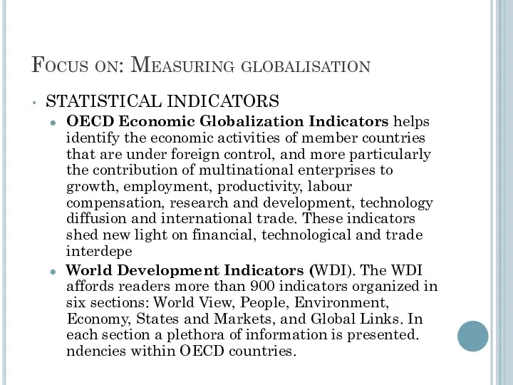
- 122. Focus on: Measuring globalisation STATISTICAL INDICATORS OECD Economic Globalization Indicators helps identify the economic activities of
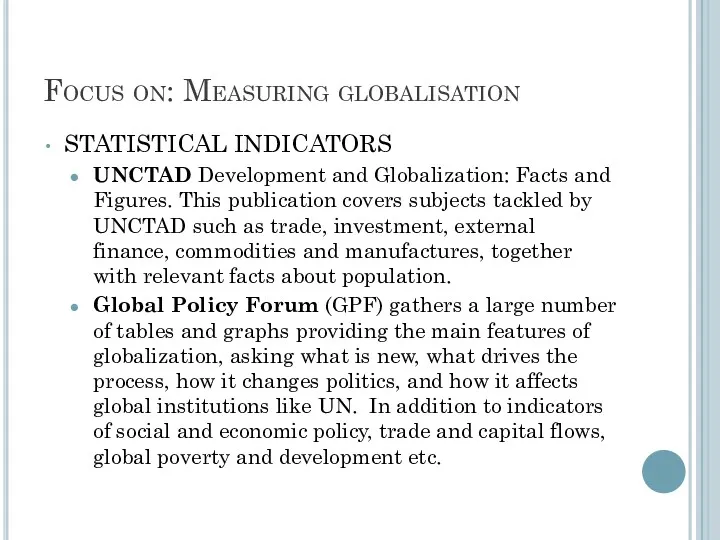
- 123. Focus on: Measuring globalisation STATISTICAL INDICATORS UNCTAD Development and Globalization: Facts and Figures. This publication covers
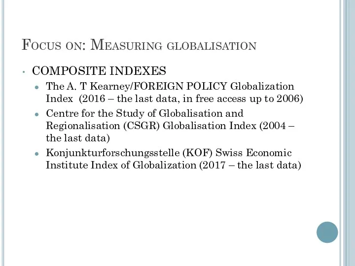
- 124. Focus on: Measuring globalisation COMPOSITE INDEXES The A. T Kearney/FOREIGN POLICY Globalization Index (2016 – the
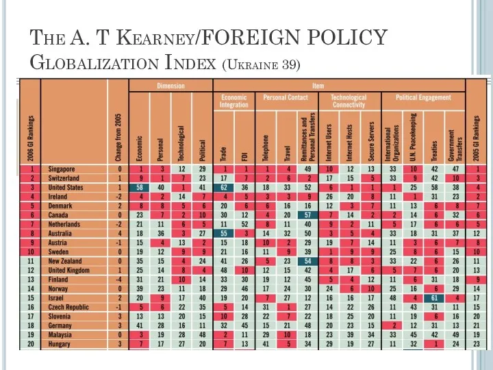
- 125. The A. T Kearney/FOREIGN POLICY Globalization Index (Ukraine 39)
- 126. CSGR Globalisation Index
- 127. KOF Globalization Index - 100 most globalized countries 2017
- 128. Methodology
- 129. Methodology
- 130. Methodology POLITICAL GLOBALIZATION [27%] Embassies in Country (25%) Membership in International Organizations (27%) Participation in U.N.
- 131. “Arguably no other place on earth has so engineered itself to prosper from globalization - and
- 132. Economic dimension Growing economic interdependence of countries worldwide through increasing volume and variety of cross-border transactions
- 133. Tow types globalization
- 134. Measuring globalization (economic aspects) Statistics related to trade. Total exports, total trade (imports + exports), Trade
- 135. Factors which help the spread of globalisation Low transport costs, containerization Telecommunications Internet Low trade barriers
- 136. Increased competition among nations For example, many companies have shifted their production facilities to emerging markets
- 137. Increased competition among nations “They (economists) predict that increased competition from low-wage countries will destroy jobs
- 138. Widening income gap For example, with improved communications and transportation, business owners in developed countries are
- 139. Pros and Cons of Globalization Free trade is supposed to reduce barriers such as tariffs, value
- 140. Pros & Cons According to supporters globalization and democracy should go hand in hand. It should
- 141. Pros & Cons Socially we have become more open and tolerant towards each other and people
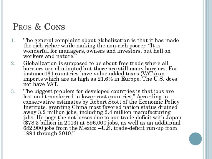
- 142. Pros & Cons The general complaint about globalization is that it has made the rich richer
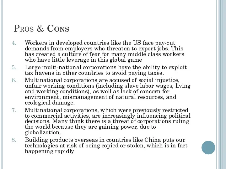
- 143. Pros & Cons Workers in developed countries like the US face pay-cut demands from employers who
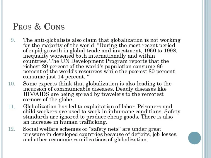
- 144. Pros & Cons The anti-globalists also claim that globalization is not working for the majority of
- 145. Documentory
- 146. GDP (2016)
- 147. GDP per capita (2016)
- 148. Macroeconomics Productivity, Output & Employment Zharova Liubov Zharova_l@ua.fm
- 149. How much does the economy produce? The quantity that an economy will produce depends on two
- 150. Factors affecting productivity Technology Inputs Labor Capital Land Raw materials Machinery Power Time period
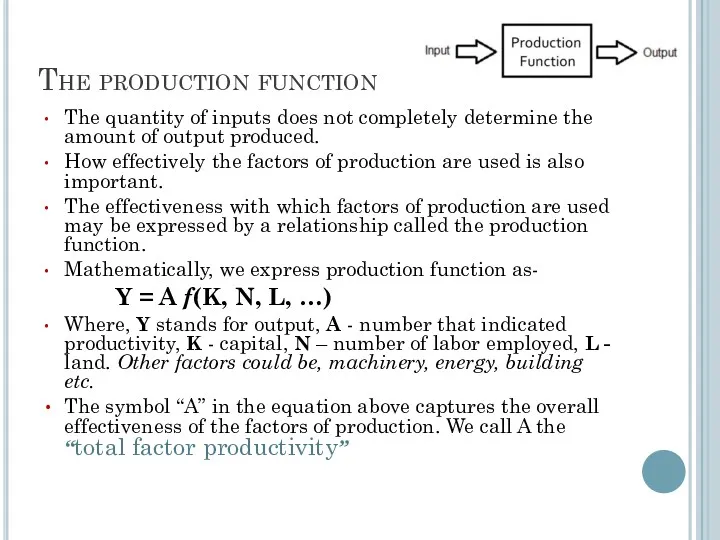
- 151. The production function The quantity of inputs does not completely determine the amount of output produced.
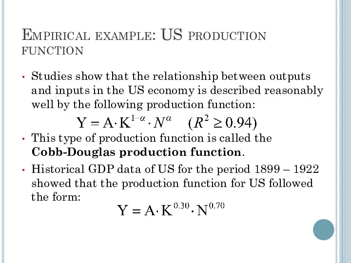
- 152. Empirical example: US production function Studies show that the relationship between outputs and inputs in the
- 153. Calculating “A”
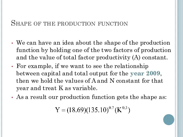
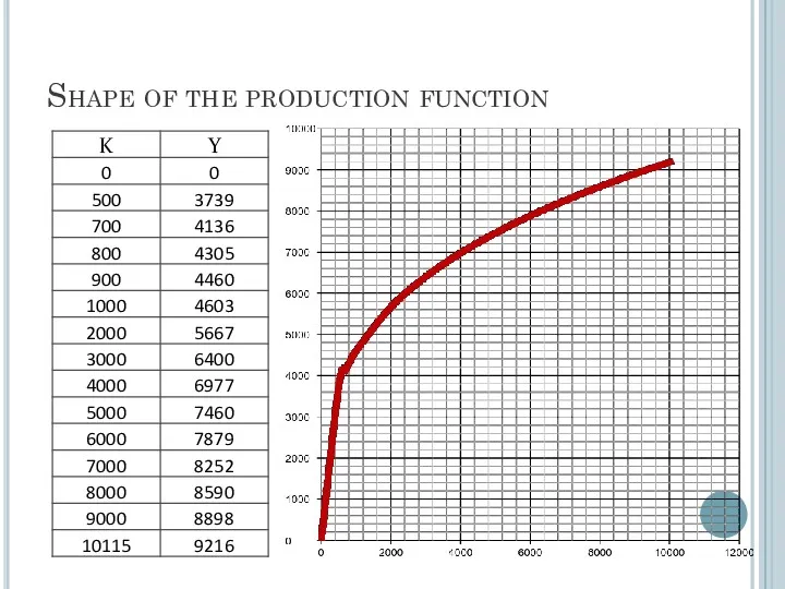
- 154. Shape of the production function We can have an idea about the shape of the production
- 155. Shape of the production function
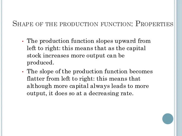
- 156. Shape of the production function: Properties The production function slopes upward from left to right: this
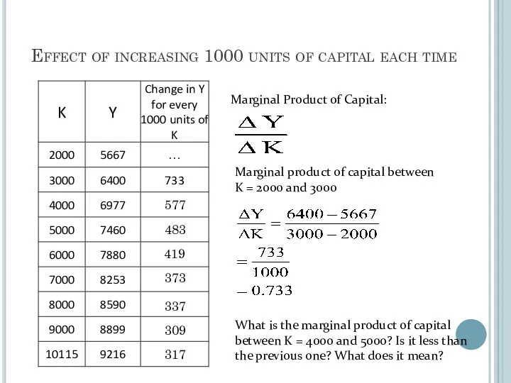
- 157. Effect of increasing 1000 units of capital each time Marginal Product of Capital: Marginal product of
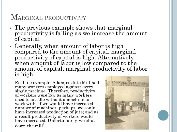
- 158. Marginal productivity The previous example shows that marginal productivity is falling as we increase the amount
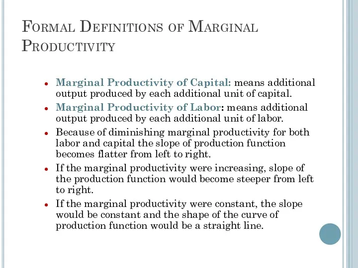
- 159. Formal Definitions of Marginal Productivity Marginal Productivity of Capital: means additional output produced by each additional
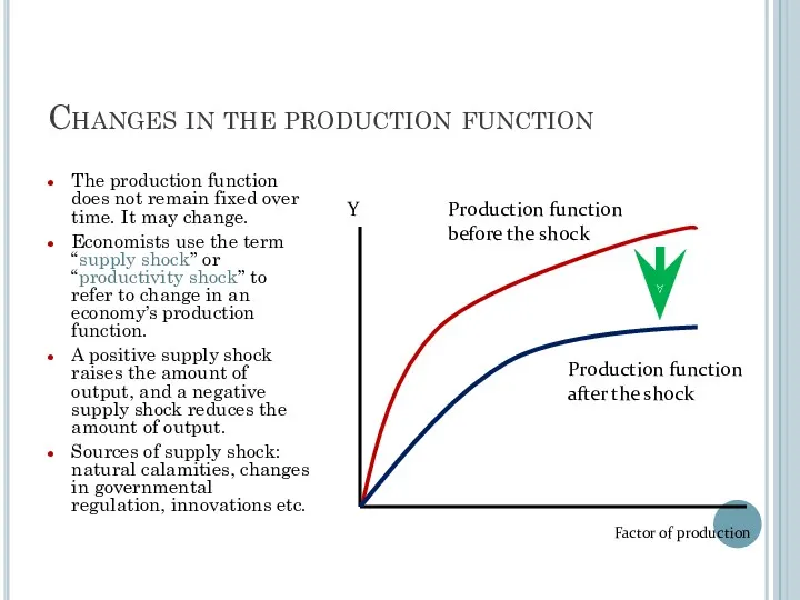
- 160. Changes in the production function The production function does not remain fixed over time. It may
- 161. Demand for labor In contrast to the amount of capital, the amount of labor employed in
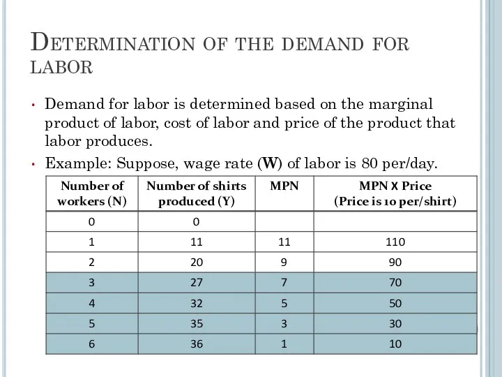
- 162. Determination of the demand for labor Demand for labor is determined based on the marginal product
- 163. Determination of demand for labor To maximize profit the firm will follow the following rules: The
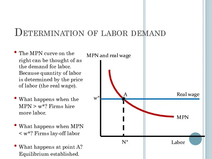
- 164. Determination of labor demand w* N* MPN and real wage Labor MPN Real wage The MPN
- 165. Factors that shift labor demand curve Changes in the wage do not shift the labor demand
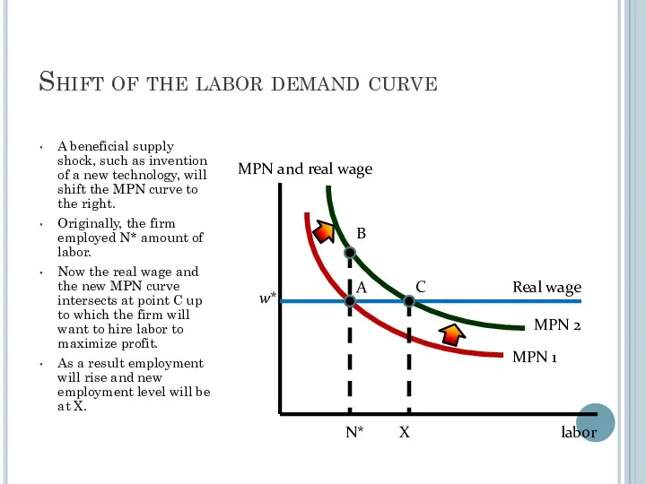
- 166. Shift of the labor demand curve A beneficial supply shock, such as invention of a new
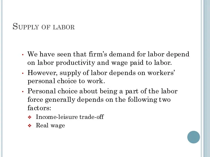
- 167. Supply of labor We have seen that firm’s demand for labor depend on labor productivity and
- 168. Labor supply curve Labor supply curve looks the same as the supply curve we studied before.
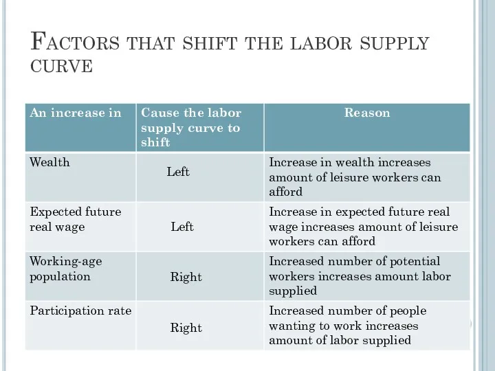
- 169. Factors that shift the labor supply curve Left Left Right Right
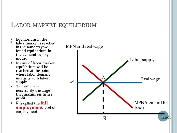
- 170. Labor market equilibrium w* MPN and real wage labor MPN/demand for labor Real wage A Labor
- 171. When profit maximizing wage is higher than equilibrium wage Labor market equilibrium is at point A.
- 172. Effects of adverse supply shock W2 N2 real wage labor ND 1 B N1 ND2 A
- 173. What if all workers are not alike? We assumed that all workers are alike. By this,
- 174. Unemployment: the untold story of full-employment Full-employment level implies that all the workers who are willing
- 175. Productivity / GDP per capita & GDP (PPP) Prof. Zharova Liubov Zharova_l@ua.fm
- 176. GDP Per Capita / GDP PPP (purchasing parity power) GDP per capita = GDP / Population
- 177. Why do we need GDP per capita? sometimes used as an indicator of standard of living,
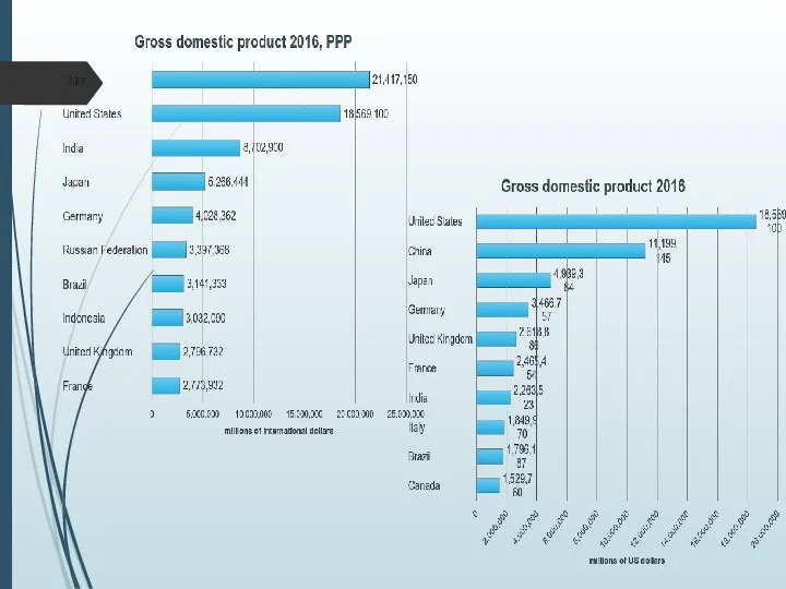
- 178. GDP (2016) GDP per capita (2016)
- 179. Why do we need GDP per capita? can also be used to measure the productivity of
- 180. The most productive countries (2015) NB: Working longer hours doesn't necessarily result in increased productivity. Mexico—the
- 182. Labour productivity Labour productivity is defined as real gross domestic product (GDP) per hour worked. This
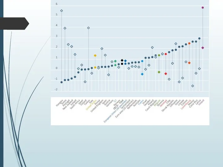
- 184. Labour productivity and utilization Labour productivity growth is a key dimension of economic performance and an
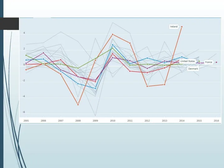
- 186. Multifactor productivity Multifactor productivity (MFP) reflects the overall efficiency with which labour and capital inputs are
- 188. What Is Purchasing Power Parity? Macroeconomic analysis relies on several different metrics to compare economic productivity
- 189. PPP calculation Problem: To make a comparison of prices across countries that holds any type of
- 190. The Big Mac Index: an example of PPP (The Economist) Prehistory: The Economist has tracked the
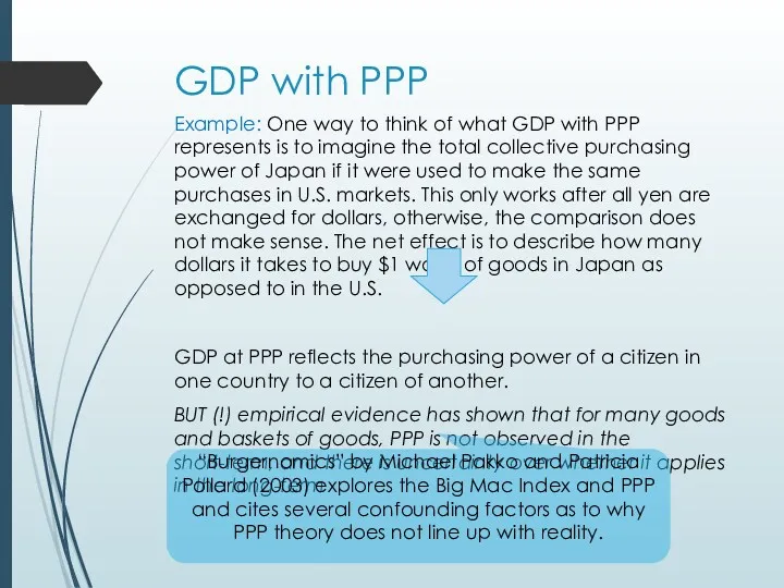
- 192. GDP with PPP Example: One way to think of what GDP with PPP represents is to
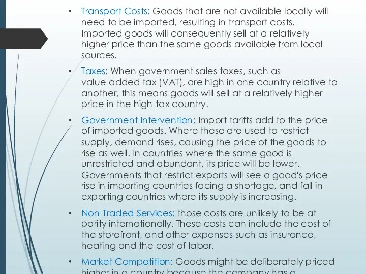
- 193. Transport Costs: Goods that are not available locally will need to be imported, resulting in transport
- 194. Venezuela case
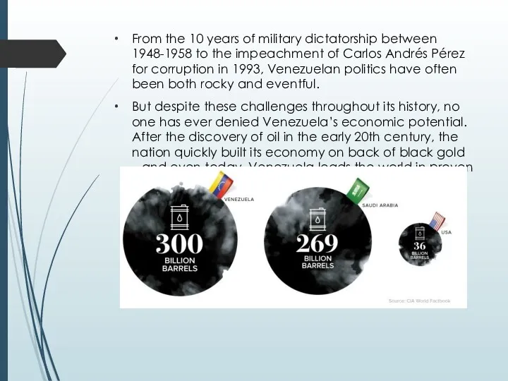
- 195. From the 10 years of military dictatorship between 1948-1958 to the impeachment of Carlos Andrés Pérez
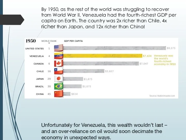
- 196. By 1950, as the rest of the world was struggling to recover from World War II,
- 197. The Downfall of Venezuela’s Economy From 1950 to the early 1980s, the Venezuelan economy experienced steady
- 199. Although oil revenues are tempting to rely on to maintain social order, they come with a
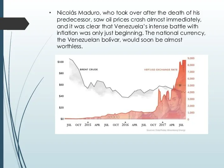
- 200. The graphic shows Venezuela’s oil revenues (in 2000 dollars) against the rate of inflation – and
- 201. Nicolás Maduro, who took over after the death of his predecessor, saw oil prices crash almost
- 202. The details of today’s crisis and intense hyperinflation are widely shared. (http://money.visualcapitalist.com/trajectory-venezuelan-hyperinflation-familiar/) The country has massive
- 203. Macroeconomics Consumption, Savings & Investment Zharova Liubov Zharova_l@ua.fm
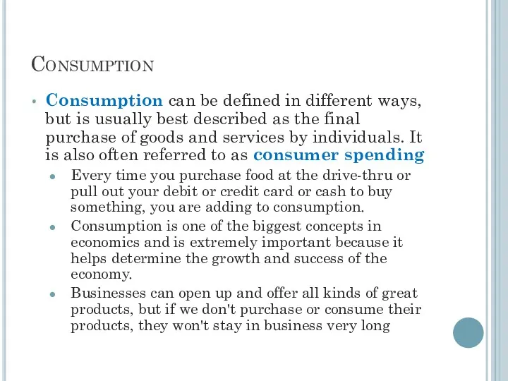
- 204. Consumption Consumption can be defined in different ways, but is usually best described as the final
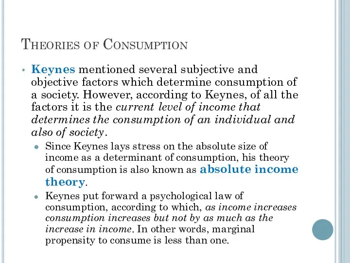
- 205. Theories of Consumption Keynes mentioned several subjective and objective factors which determine consumption of a society.
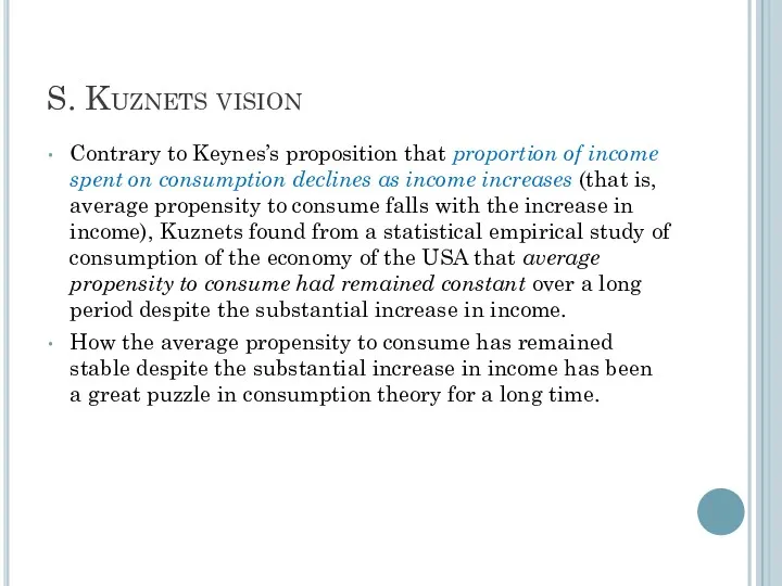
- 206. S. Kuznets vision Contrary to Keynes’s proposition that proportion of income spent on consumption declines as
- 208. Relative Income Theory of Consumption (J.S. Duesenberry) Assumptions: the determinant of consumption is relative income of
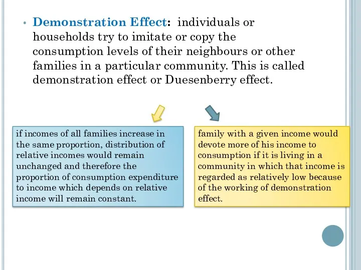
- 209. Demonstration Effect: individuals or households try to imitate or copy the consumption levels of their neighbours
- 210. Ratchet Effect - when income of individuals or households falls, their consumption expenditure does not fall
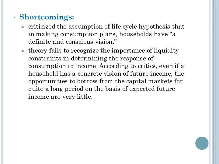
- 211. Life Cycle Theory of Consumption ( Albert Ando & Franco Modigliani) Idea: the consumption in any
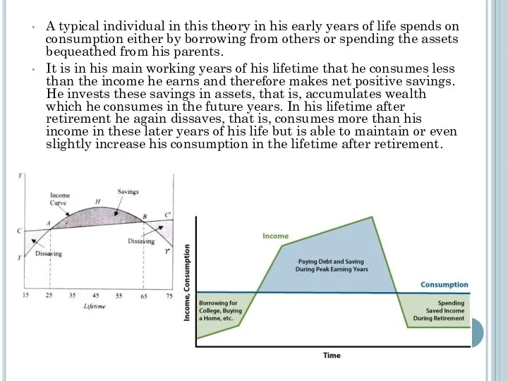
- 212. A typical individual in this theory in his early years of life spends on consumption either
- 213. Shortcomings: criticized the assumption of life cycle hypothesis that in making consumption plans, households have “a
- 214. Permanent Income Theory of Consumption (Milton Friedman) Assumptions: consumption is determined by long-term expected income (permanent
- 215. Relationship between Consumption and Permanent Income: Cp = k(i,w,u) ×Yp Cp – permanent consumption; Yp –
- 216. In addition to permanent income (Yp), the individual’s income may contain a transitory component - transitory
- 217. Conclusions: Permanent income hypothesis is similar to life cycle hypothesis and differs only in details Permanent
- 218. Real income vs. nominal income The term 'real' that is used in describing income refers to
- 219. Savings Savings, according to Keynesian economics, consists of the amount left over when the cost of
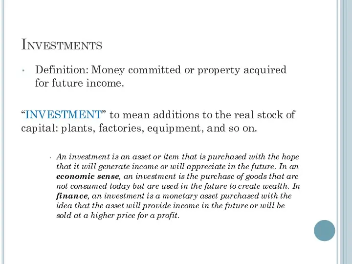
- 221. Investments Definition: Money committed or property acquired for future income. “INVESTMENT” to mean additions to the
- 222. Leverage Firms (Companies), are the best place to invest, because it’s Earning per share is high.
- 224. Final Conclusions Consumed is what you buy or ability to pay. High consumption makes any product
- 225. Macroeconomics GDP Income Economic Growth Zharova Liubov
- 226. GDP = is the monetary value of all the finished goods and services produced within a
- 227. Approaches to calculate GDP Expenditure & Income Methods Expenditure Method – count all new goods &
- 236. Expenditure approach for 1 product economy Roaster Wages $15,000 Taxes $5,000 Revenue $35,000 beans sold to
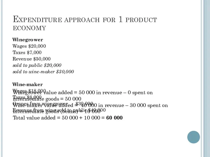
- 237. Expenditure approach for 1 product economy Winegrower Wages $20,000 Taxes $7,000 Revenue $50,000 sold to public
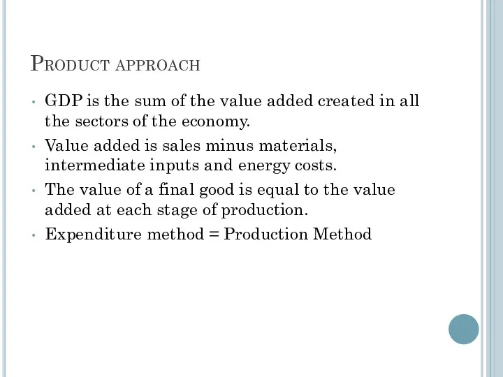
- 238. Product approach GDP is the sum of the value added created in all the sectors of
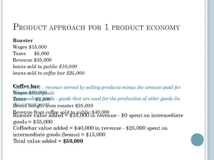
- 239. Product approach for 1 product economy Roaster Wages $15,000 Taxes $5,000 Revenue $35,000 beans sold to
- 240. Expenditure approach for 1 product economy Winegrower Wages $20,000 Taxes $7,000 Revenue $50,000 sold to public
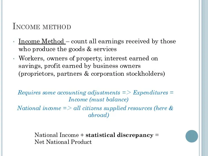
- 241. Income method Income Method – count all earnings received by those who produce the goods &
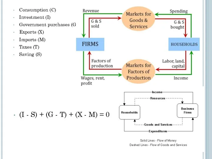
- 242. Consumption (C) Investment (I) Government purchases (G) Exports (X) Imports (M) Taxes (T) Saving (S) (I
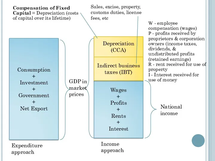
- 243. Consumption + Investment + Government + Net Export Wages + Profits + Rents + Interest Depreciation
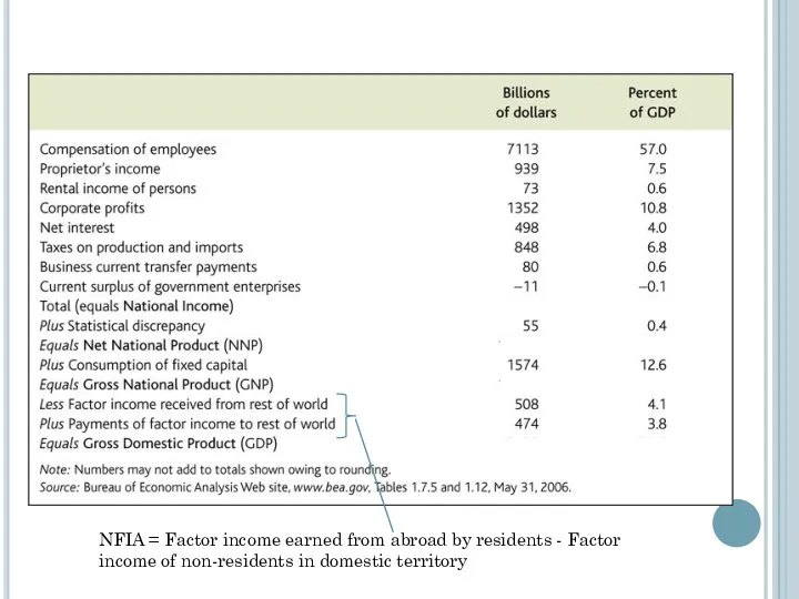
- 244. NFIA = Factor income earned from abroad by residents - Factor income of non-residents in domestic
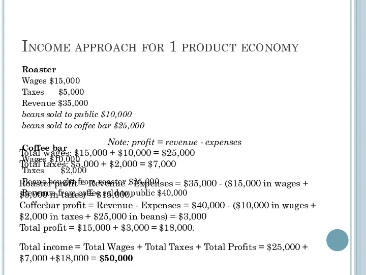
- 246. Income approach for 1 product economy Roaster Wages $15,000 Taxes $5,000 Revenue $35,000 beans sold to
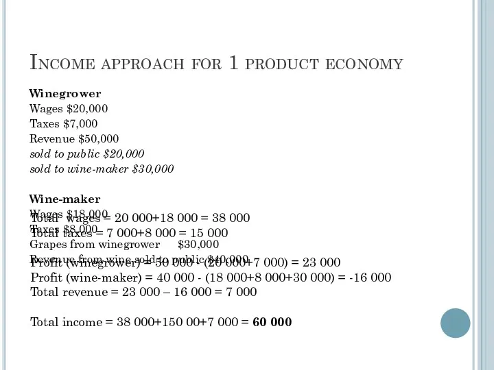
- 247. Income approach for 1 product economy Winegrower Wages $20,000 Taxes $7,000 Revenue $50,000 sold to public
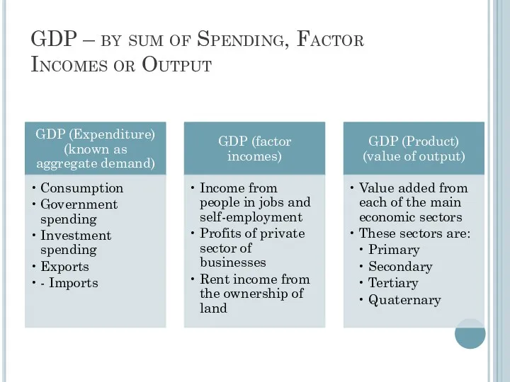
- 248. GDP – by sum of Spending, Factor Incomes or Output
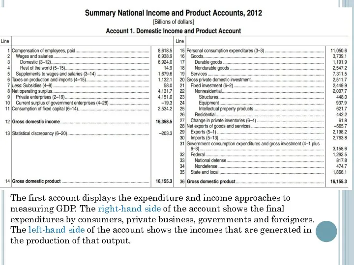
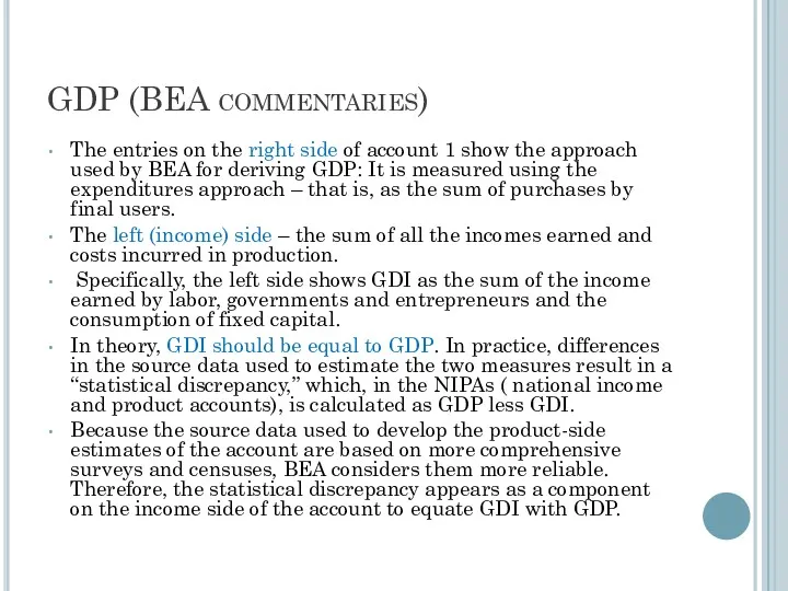
- 249. The first account displays the expenditure and income approaches to measuring GDP. The right-hand side of
- 250. GDP (BEA commentaries) The entries on the right side of account 1 show the approach used
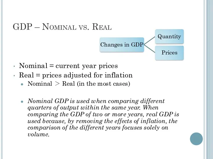
- 252. GDP – Nominal vs. Real Nominal = current year prices Real = prices adjusted for inflation
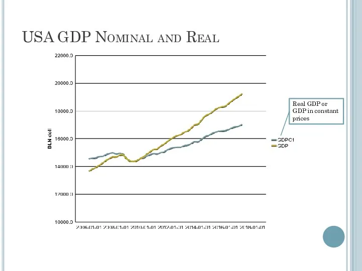
- 253. USA GDP Nominal and Real Real GDP or GDP in constant prices
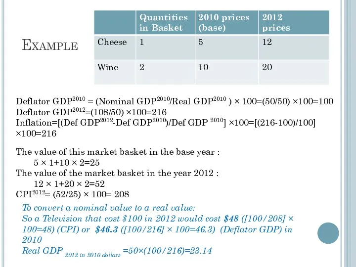
- 255. Example Nominal GDP =Pcheese∗QCheese+Pcheese∗QCheese Nominal GDP =Pcheese∗Qcheese+Pwine∗Qwine Nominal GDP2010 = 5*2+10*4=50 Nominal GDP2011=12*3+17*3=87 Nominal GDP2012=12*4+20*3=108 Real
- 256. where GDPt is the level of activity in the later period; GDP0 is the level of
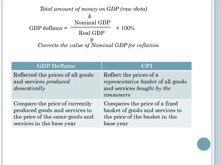
- 257. Deflator GDP GDP deflator is an index of the price level relative to some base year.
- 258. GDP deflator = Nominal GDP Real GDP × 100% Total amount of money on GDP (raw
- 259. What is the relationship between GDP deflator & CPI? Both GDP deflator and CPI are measures
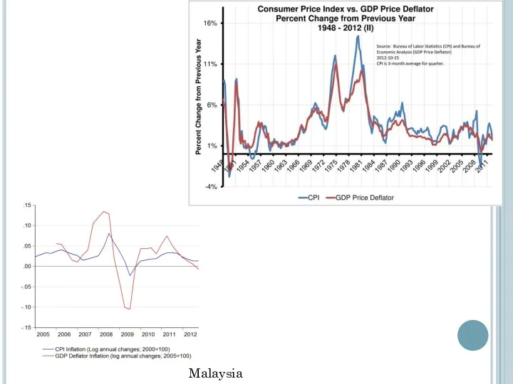
- 260. Malaysia
- 261. Example The value of this market basket in the base year : 5 × 1+10 ×
- 262. Define Inflation as the growth rate of prices. The greek letter π is often used as
- 263. Macroeconomics GDP /Business Cycle Unemployment Zharova Liubov
- 264. Example In 1966, Howard Hughes was forced to sell TWA (trans world airlines) and received a
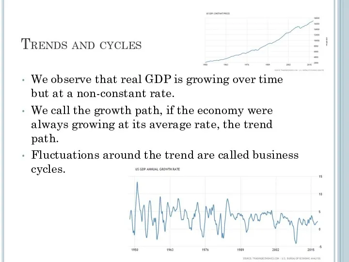
- 265. Trends and cycles We observe that real GDP is growing over time but at a non-constant
- 266. Business Cycle term As the economy fluctuates around the trend, the economy is experiencing business cycles.
- 267. The correlation of business cycles implies that groups of countries are in the same phase for
- 268. North American Free Trade Agreement (NAFTA) It is a piece of regulation implemented January 1, 1994
- 269. The global expansion remains relatively steady and synchronized across major economies. Broadly speaking, most developed economies
- 270. Recession and booms Business cycle positions are sometimes characterized as booms and recessions. These names have
- 271. Hong Kong Business Cycle
- 272. Business Cycles & Co-movement Business cycles are fluctuations in the economy as a whole. Different sub-categories
- 273. Business Cycles & Sub-Categories Expenditure. Consumption and Investment co-move with output. Investment is more volatile than
- 274. Hong Kong Expenditure Cycle
- 275. Corporate Profits Corporate profits are strongly pro-cyclical and volatile. When the economy is doing well, corporations
- 276. Using financial market data to predict business cycles It has been joked that stock markets have
- 277. The traditional business cycle frequency is around one to eight years. By contrast, the financial cycles
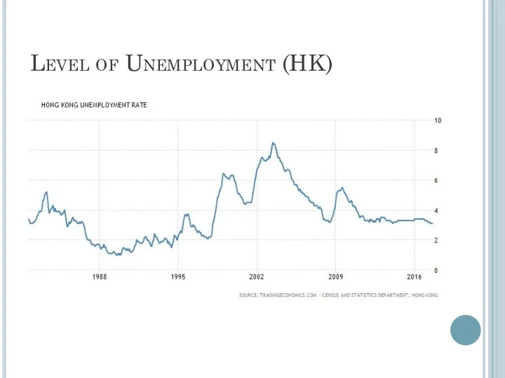
- 279. Level of Unemployment (HK)
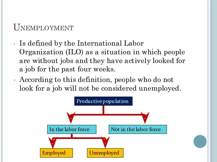
- 280. Unemployment Is defined by the International Labor Organization (ILO) as a situation in which people are
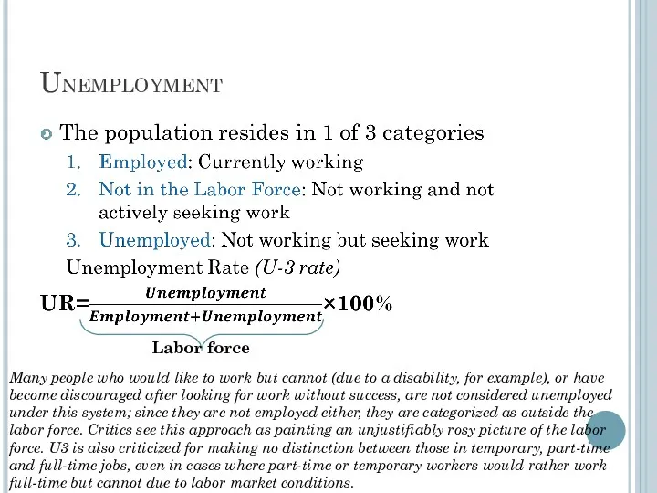
- 281. Unemployment Labor force Many people who would like to work but cannot (due to a disability,
- 282. Employment dynamics Employed labor force Unemployed New hire/ recall Lay off/ quits Out of the labor
- 283. Example Who is counted as employed? On vacation Ill Experiencing child care problems On maternity or
- 284. Example Garrett is 16 years old, and he has no job from which he receives any
- 285. Types of Unemployment
- 286. Underemployment Underemployment is a measure of employment and labor utilization in the economy that looks at
- 287. Disguised (hidden) Unemployment Disguised unemployment exists where part of the labor force is either left without
- 288. Alternative Measures U-1 People who have been unemployed for 15 weeks or longer, expressed as a
- 289. Alternative Measures U-5 Unemployed people, plus those who are marginally attached to the labor force, as
- 290. Alternative Measures U-6 Unemployed people, plus people who are marginally attached to the labor force, plus
- 292. Tightly regulated labor markets increase structural unemployment. High social welfare benefits increase frictional costs as workers
- 293. How to solve the problem There are two ways the government can help the unemployed. There
- 294. Macroeconomics aggregated supply and demand Zharova Liubov
- 295. Aggregate Demand (AD) Aggregate demand is the total demand for goods and services is an economic
- 296. AD shifts AD = C+I+G+NX change in consumption (eg cut tax) Or tax increasing Shifts in
- 297. Components of AS Consumer goods. Private consumer goods and services, such as motor vehicles, computers, clothes
- 298. Long-run Aggregate supply (LRAS) Supply = capability to produce Population growth Easy to find a job
- 299. Sort-run Aggregate Supply (SRAS) Rising the price – labor pool, work more, less vacation… Decreasing price
- 300. Summirising Aggregate supply is the total quantity of output firms will produce and sell – in
- 301. Equilibrium in the aggregate demand/aggregate supply model At a relatively low price level for output, firms
- 302. Price level: aggregate demand/aggregate supply Conclusions: the equilibrium is fairly far from where the AS curve
- 303. Example Bebebe. The imaginary country of Bebebe has the aggregate supply and aggregate demand curves given
- 304. How productivity growth shifts the AS curve Over time, productivity grows so that the same quantity
- 306. Summary The aggregate demand/aggregate supply model is a model that shows what determines total supply or
- 307. How do changes by consumers and firms affect AD? When consumers feel more confident about the
- 308. Government macroeconomic policy choices can shift AD. Take, for example, government spending–one component of AD. Higher
- 309. During a recession, when unemployment is high and many businesses are suffering low profits or even
- 311. Скачать презентацию
Economy…
. . . The word economy comes from a Greek word
Economy…
. . . The word economy comes from a Greek word
PRINCIPLES OF ECONOMICS
A household and an economy face many decisions:
Who will
PRINCIPLES OF ECONOMICS
A household and an economy face many decisions:
Who will
PRINCIPLES OF ECONOMICS
Society and Scarce Resources:
The management of society’s resources is
PRINCIPLES OF ECONOMICS
Society and Scarce Resources:
The management of society’s resources is
Economics
Economics is the study of how society manages its scarce resources.
The
Economics
Economics is the study of how society manages its scarce resources.
The
10 PRINCIPLES OF ECONOMICS
How people make decisions.
People face tradeoffs.
The cost of
10 PRINCIPLES OF ECONOMICS
How people make decisions.
People face tradeoffs.
The cost of
10 PRINCIPLES OF ECONOMICS
How people interact with each other.
Trade can make
10 PRINCIPLES OF ECONOMICS
How people interact with each other.
Trade can make
10 PRINCIPLES OF ECONOMICS
The forces and trends that affect how the
10 PRINCIPLES OF ECONOMICS
The forces and trends that affect how the

Principle #1: People Face Tradeoffs
Trade off is a situation that involves
Principle #1: People Face Tradeoffs
Trade off is a situation that involves
Principle #1: People Face Tradeoffs
To get one thing, we usually have
Principle #1: People Face Tradeoffs
To get one thing, we usually have
Principle #1: People Face Tradeoffs
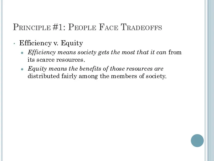
Efficiency v. Equity
Efficiency means society gets the
Principle #1: People Face Tradeoffs
Efficiency v. Equity
Efficiency means society gets the
Principle #2: The Cost of Something Is What You Give Up
Principle #2: The Cost of Something Is What You Give Up

Principle #2: The Cost of Something Is What You Give Up
Principle #2: The Cost of Something Is What You Give Up
Principle #3: Rational People Think at the Margin
Rational people people who
Principle #3: Rational People Think at the Margin
Rational people people who

Principle #4: People Respond to Incentives
Incentives – something that induces a
Principle #4: People Respond to Incentives
Incentives – something that induces a
Principle #5: Trade Can Make Everyone
Better Off
People gain from their ability
Principle #5: Trade Can Make Everyone
Better Off
People gain from their ability
Principle #6: Markets Are Usually a Good Way to Organize Economic
Principle #6: Markets Are Usually a Good Way to Organize Economic
Principle #6: Markets Are Usually a Good Way to Organize Economic
Principle #6: Markets Are Usually a Good Way to Organize Economic
Principle #7: Governments Can Sometimes Improve Market Outcomes
Market failure occurs when
Principle #7: Governments Can Sometimes Improve Market Outcomes
Market failure occurs when
Principle #7: Governments Can Sometimes Improve Market Outcomes
Market failure may be
Principle #7: Governments Can Sometimes Improve Market Outcomes
Market failure may be
Principle #8: The Standard of Living Depends on a Country’s Production
Standard
Principle #8: The Standard of Living Depends on a Country’s Production
Standard
Principle #8: The Standard of Living Depends on a Country’s Production
Almost
Principle #8: The Standard of Living Depends on a Country’s Production
Almost
Principle #9: Prices Rise When the
Government Prints Too Much Money
Inflation is
Principle #9: Prices Rise When the
Government Prints Too Much Money
Inflation is
Principle #10: Society Faces a Short-run
Tradeoff Between Inflation and Unemployment
It’s a
Principle #10: Society Faces a Short-run
Tradeoff Between Inflation and Unemployment
It’s a
Summary
When individuals make decisions, they face tradeoffs among alternative goals.
The cost
Summary
When individuals make decisions, they face tradeoffs among alternative goals.
The cost
Summary
Trade can be mutually beneficial.
Markets are usually a good way of
Summary
Trade can be mutually beneficial.
Markets are usually a good way of
Summary
Productivity is the ultimate source of living standards.
Money growth is the
Summary
Productivity is the ultimate source of living standards.
Money growth is the
Macroeconomics
Introduction to Macroeconomics
Zharova Liubov
Zharova_l@ua.fm
Macroeconomics
Introduction to Macroeconomics
Zharova Liubov
Zharova_l@ua.fm
Intro
individual decision-making Microeconomics examines the behavior of units—business firms and households.
Macroeconomics
Intro
individual decision-making Microeconomics examines the behavior of units—business firms and households.
Macroeconomics
Intro
When we study the consumption behaviour or equilibrium of a consumer;
Intro
When we study the consumption behaviour or equilibrium of a consumer;
Intro
Microeconomists generally conclude that markets work well.
Macroeconomists, however, observe that some
Intro
Microeconomists generally conclude that markets work well.
Macroeconomists, however, observe that some
Intro
Macroeconomists often reflect on the microeconomic principles underlying macroeconomic analysis, or
Intro
Macroeconomists often reflect on the microeconomic principles underlying macroeconomic analysis, or
The Roots of Macroeconomics
The Great Depression was a period of severe
The Roots of Macroeconomics
The Great Depression was a period of severe
The Roots of Macroeconomics
Classical economists applied microeconomic models, or “market clearing”
The Roots of Macroeconomics
Classical economists applied microeconomic models, or “market clearing”
The Roots of Macroeconomics
In 1936, John Maynard Keynes published The General
The Roots of Macroeconomics
In 1936, John Maynard Keynes published The General
Recent Macroeconomic History
Fine-tuning was the phrase used by Walter Heller to
Recent Macroeconomic History
Fine-tuning was the phrase used by Walter Heller to
Why to Study Macroeconomics?
Macroeconomics is the study of the nation’s economy
Why to Study Macroeconomics?
Macroeconomics is the study of the nation’s economy
Macroeconomic Concerns
Three of the major concerns of macroeconomics are:
Inflation
Output growth
Unemployment
Macroeconomic Concerns
Three of the major concerns of macroeconomics are:
Inflation
Output growth
Unemployment
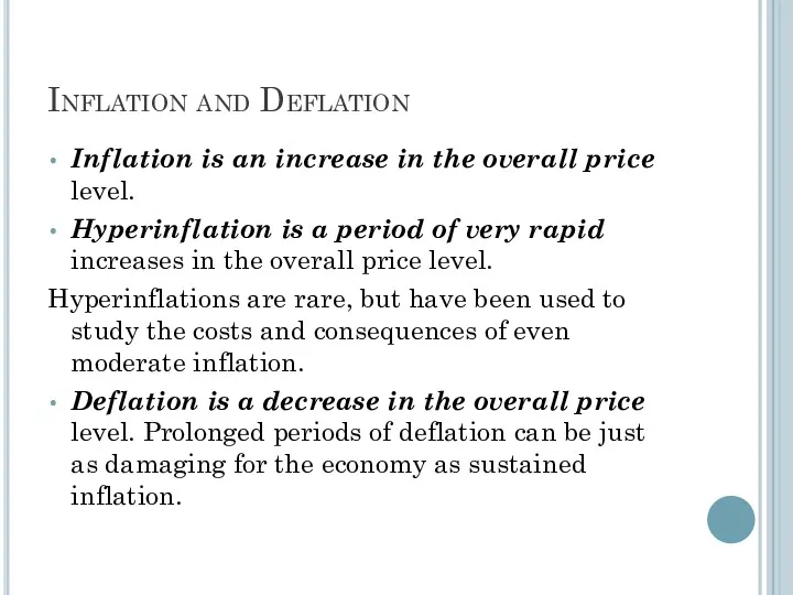
Inflation and Deflation
Inflation is an increase in the overall price level.
Hyperinflation
Inflation and Deflation
Inflation is an increase in the overall price level.
Hyperinflation
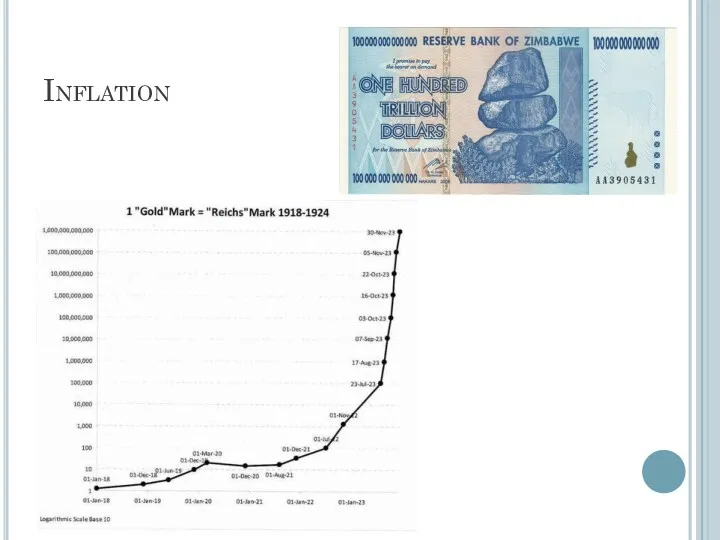
Inflation
Inflation
Output Growth:
Short Run and Long Run
The business cycle is the
Output Growth:
Short Run and Long Run
The business cycle is the
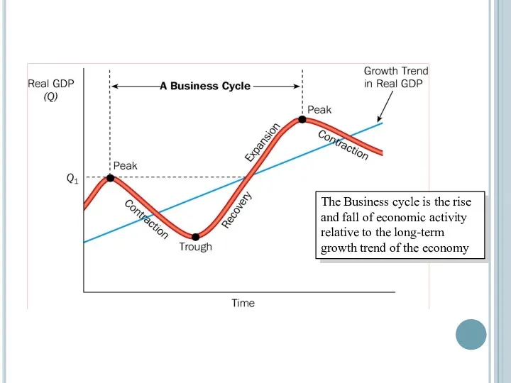
The Business cycle is the rise and fall of economic activity
The Business cycle is the rise and fall of economic activity
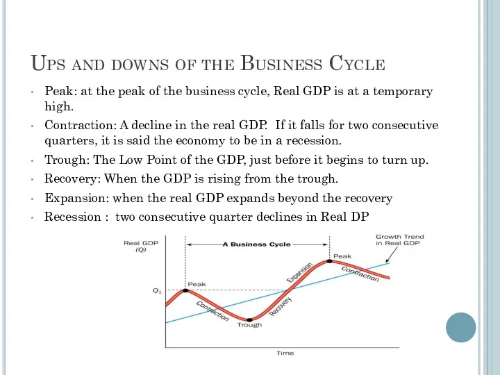
Ups and downs of the Business Cycle
Peak: at the peak of
Ups and downs of the Business Cycle
Peak: at the peak of
Recent Macroeconomic History
Stagflation occurs when the overall price level rises rapidly
Recent Macroeconomic History
Stagflation occurs when the overall price level rises rapidly
Stagflation
Stagflation is a contraction of a nation’s output accompanied by inflation
Staglation
Stagflation
Stagflation is a contraction of a nation’s output accompanied by inflation
Staglation
Output Growth:
Short Run and Long Run
A recession is a period during
Output Growth:
Short Run and Long Run
A recession is a period during
Unemployment
The unemployment rate is the percentage of the labor force that
Unemployment
The unemployment rate is the percentage of the labor force that
Unemployment
Unemployment
Government in the Macroeconomy
There are three kinds of policy that the
Government in the Macroeconomy
There are three kinds of policy that the
Government in the Macroeconomy
Fiscal policy refers to government policies concerning taxes
Government in the Macroeconomy
Fiscal policy refers to government policies concerning taxes
The Components of the Macroeconomy
The circular flow diagram shows the income
The Components of the Macroeconomy
The circular flow diagram shows the income
The Components of the Macroeconomy
The Components of the Macroeconomy
The Components of the Macroeconomy
The Components of the Macroeconomy
The Components of the Macroeconomy
Transfer payments are payments made by the
The Components of the Macroeconomy
Transfer payments are payments made by the
The Three Market Arenas
Households, firms, the government, and the rest of
The Three Market Arenas
Households, firms, the government, and the rest of
The Three Market Arenas
Households and the government purchase goods and services
The Three Market Arenas
Households and the government purchase goods and services
The Three Market Arenas
In the money market – sometimes called the
The Three Market Arenas
In the money market – sometimes called the
Financial Instruments
Treasury bonds, notes, and bills are promissory notes issued by
Financial Instruments
Treasury bonds, notes, and bills are promissory notes issued by
The Methodology of Macroeconomics
Connections to microeconomics:
Macroeconomic behavior is the sum of
The Methodology of Macroeconomics
Connections to microeconomics:
Macroeconomic behavior is the sum of
Aggregate Supply and
Aggregate Demand
Aggregate demand is the total demand for goods
Aggregate Supply and
Aggregate Demand
Aggregate demand is the total demand for goods
Expansion and Contraction:
The Business Cycle
An expansion, or boom, is the period
Expansion and Contraction:
The Business Cycle
An expansion, or boom, is the period
Review Terms and Concepts
aggregate behavior
aggregate demand
aggregate output
aggregate supply
business cycle
circular flow
contraction, recession,
Review Terms and Concepts
aggregate behavior
aggregate demand
aggregate output
aggregate supply
business cycle
circular flow
contraction, recession,
Macroeconomics
The Measurement and
Structure of the
National Economy
Zharova Liubov
Zharova_l@ua.fm
Macroeconomics
The Measurement and
Structure of the
National Economy
Zharova Liubov
Zharova_l@ua.fm
Outline
National Income Accounting: The Measurement of Production, Income, and Expenditure
Gross Domestic
Outline
National Income Accounting: The Measurement of Production, Income, and Expenditure
Gross Domestic
National Income Accounting
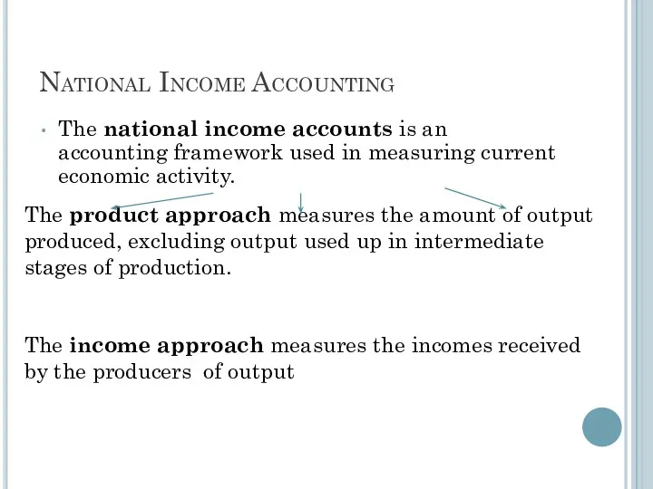
The national income accounts is an accounting framework used
National Income Accounting
The national income accounts is an accounting framework used
National Income Accounting
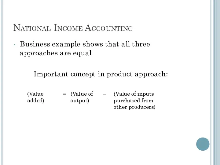
Business example shows that all three approaches are equal
Important
National Income Accounting
Business example shows that all three approaches are equal
Important
National Income Accounting
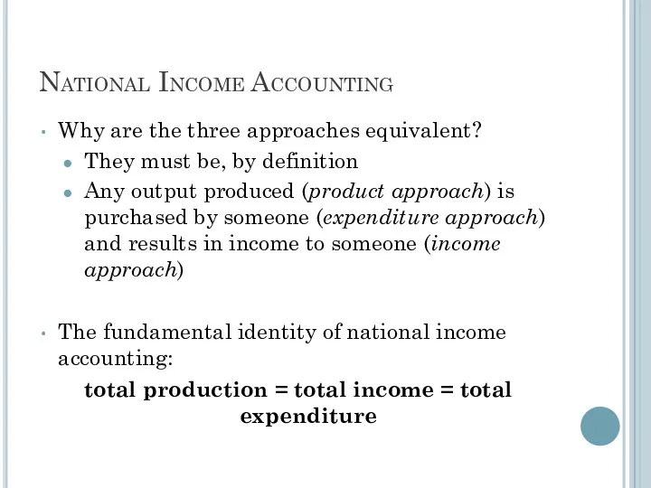
Why are the three approaches equivalent?
They must be, by
National Income Accounting
Why are the three approaches equivalent?
They must be, by
National Income Accounting
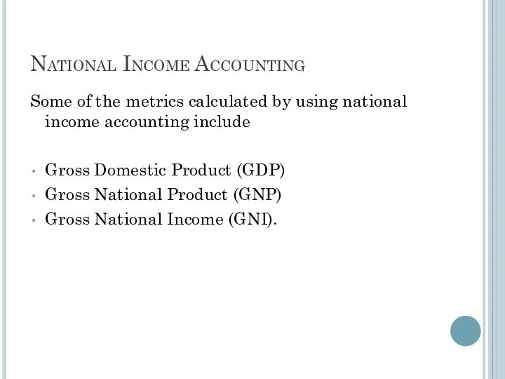
Some of the metrics calculated by using national income accounting include
Gross
National Income Accounting
Some of the metrics calculated by using national income accounting include
Gross
Gross Domestic Product
The product approach to measuring GDP
GDP (gross domestic product)
Gross Domestic Product
The product approach to measuring GDP
GDP (gross domestic product)
Gross Domestic Product
Market value: allows adding together unlike items by valuing
Gross Domestic Product
Market value: allows adding together unlike items by valuing
GDP
Newly produced: counts only things produced in the given period; excludes
GDP
Newly produced: counts only things produced in the given period; excludes
GNP
GNP (Gross National Product) = output produced by domestically owned factors
GNP
GNP (Gross National Product) = output produced by domestically owned factors
GNP
Example: Engineering revenues for a road built by a U.S. company
GNP
Example: Engineering revenues for a road built by a U.S. company
Example
If a Japanese multinational produces cars in the UK, this production
Example
If a Japanese multinational produces cars in the UK, this production
Ratio of GNP to GDP
Ukraine
China
Ratio of GNP to GDP
Ukraine
China
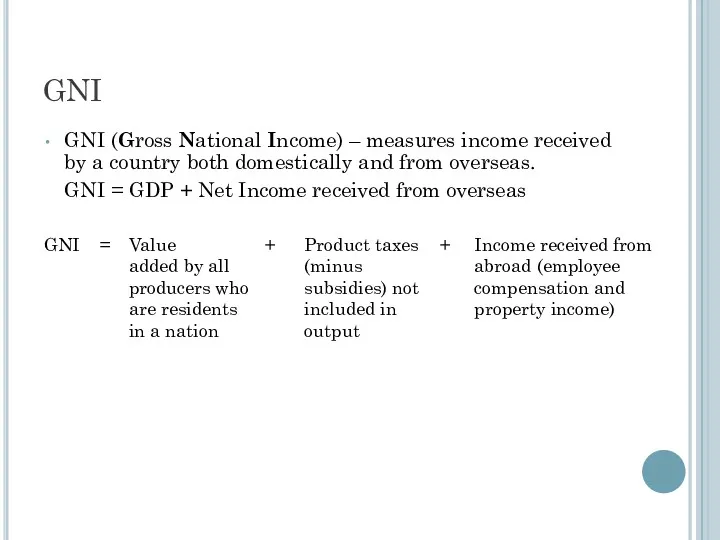
GNI
GNI (Gross National Income) – measures income received by a country
GNI
GNI (Gross National Income) – measures income received by a country
GNI
For most nations there is little difference between GDP and GNI
GNI
GNI
For most nations there is little difference between GDP and GNI
GNI
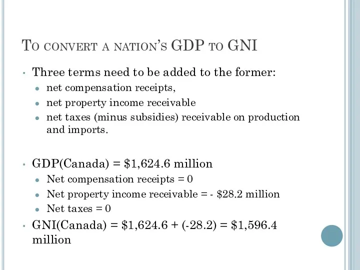
To convert a nation’s GDP to GNI
Three terms need to be
To convert a nation’s GDP to GNI
Three terms need to be
GDP measurement
The expenditure approach to measuring GDP
Measures total spending on final
GDP measurement
The expenditure approach to measuring GDP
Measures total spending on final
GDP measurement /
expenditure approach
Consumption: spending by domestic households on
GDP measurement /
expenditure approach
Consumption: spending by domestic households on
GDP measurement /
expenditure approach
Investment: spending for new capital goods
GDP measurement /
expenditure approach
Investment: spending for new capital goods
GDP measurement /
expenditure approach
Government purchases of goods and services:
GDP measurement /
expenditure approach
Government purchases of goods and services:
GDP measurement /
expenditure approach
Net exports: exports minus imports
Exports: goods
GDP measurement /
expenditure approach
Net exports: exports minus imports
Exports: goods
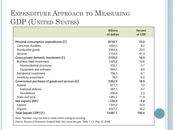
Expenditure Approach to Measuring
GDP (United States)
Expenditure Approach to Measuring
GDP (United States)
GDP measurement /
income approach
Adds up income generated by production
GDP measurement /
income approach
Adds up income generated by production
GDP measurement /
income approach
Private sector and government sector income
Private
GDP measurement /
income approach
Private sector and government sector income
Private
Income Approach to Measuring GDP (US)
Income Approach to Measuring GDP (US)
Saving and Wealth
Wealth
Household Wealth = (Household’s Assets) – (Household’s Liabilities)
National
Saving and Wealth
Wealth
Household Wealth = (Household’s Assets) – (Household’s Liabilities)
National
Saving and Wealth /
Measures of aggregate saving
Saving = Current Income
Saving and Wealth /
Measures of aggregate saving
Saving = Current Income
Saving and Wealth /
Measures of aggregate saving
Government Saving = Net
Saving and Wealth /
Measures of aggregate saving
Government Saving = Net
Saving and Wealth /
Measures of aggregate saving
National saving
National Saving =
Saving and Wealth /
Measures of aggregate saving
National saving
National Saving =
Saving and Wealth /
Measures of aggregate saving
The uses of private
Saving and Wealth /
Measures of aggregate saving
The uses of private
Saving and Wealth
The uses of private saving
Spvt = I + (–Sgovt)
Saving and Wealth
The uses of private saving
Spvt = I + (–Sgovt)
Saving and Wealth /
Relating saving and wealth
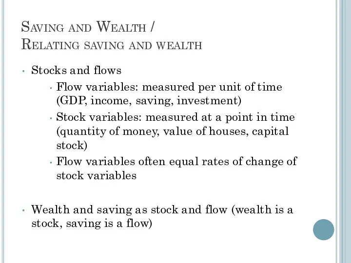
Stocks and flows
Flow variables: measured
Saving and Wealth /
Relating saving and wealth
Stocks and flows
Flow variables: measured
Saving and Wealth /
Relating saving and wealth
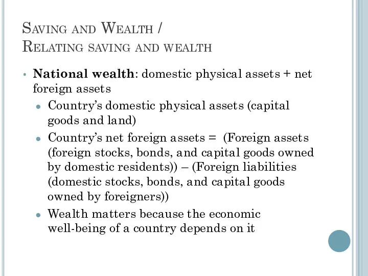
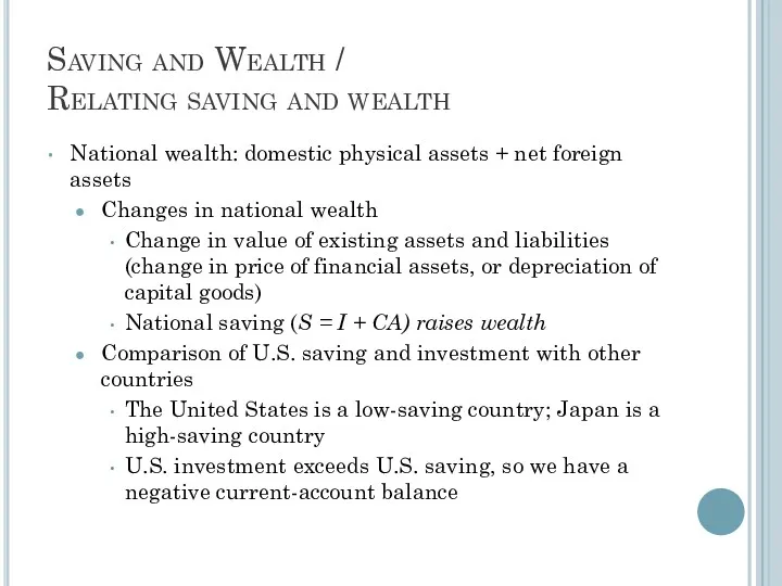
National wealth: domestic physical assets
Saving and Wealth /
Relating saving and wealth
National wealth: domestic physical assets
Saving and Wealth /
Relating saving and wealth
National wealth: domestic physical assets
Saving and Wealth /
Relating saving and wealth
National wealth: domestic physical assets
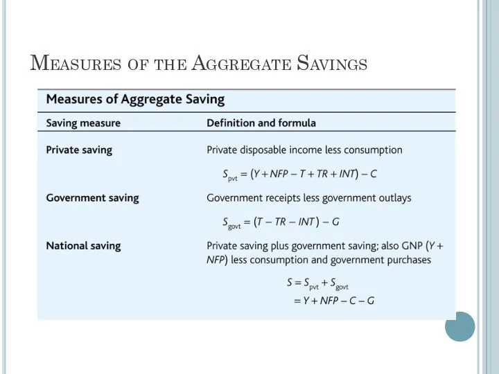
Measures of the Aggregate Savings
Measures of the Aggregate Savings
Real GDP, Price Indexes, and Inflation
Real GDP
Nominal variables are those in
Real GDP, Price Indexes, and Inflation
Real GDP
Nominal variables are those in
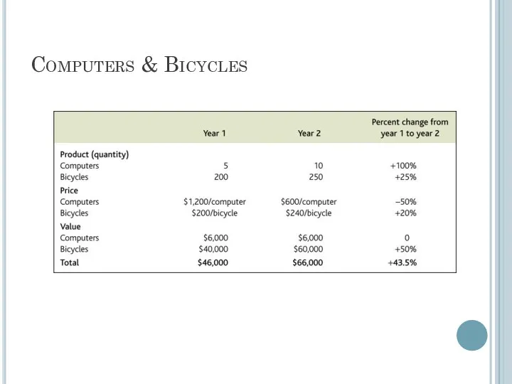
Computers & Bicycles
Computers & Bicycles
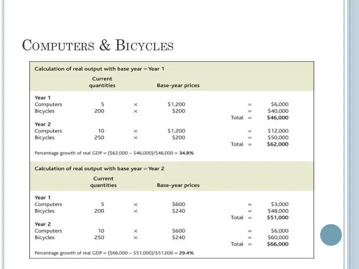
Computers & Bicycles
Computers & Bicycles
Real GDP, Price Indexes, and Inflation
Price Indexes
A price index measures the
Real GDP, Price Indexes, and Inflation
Price Indexes
A price index measures the
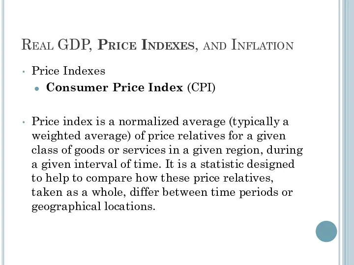
Real GDP, Price Indexes, and Inflation
Price Indexes
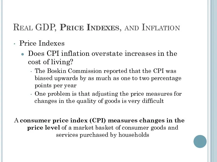
Consumer Price Index (CPI)
Price index
Real GDP, Price Indexes, and Inflation
Price Indexes
Consumer Price Index (CPI)
Price index
Real GDP, Price Indexes, and Inflation
Price Indexes
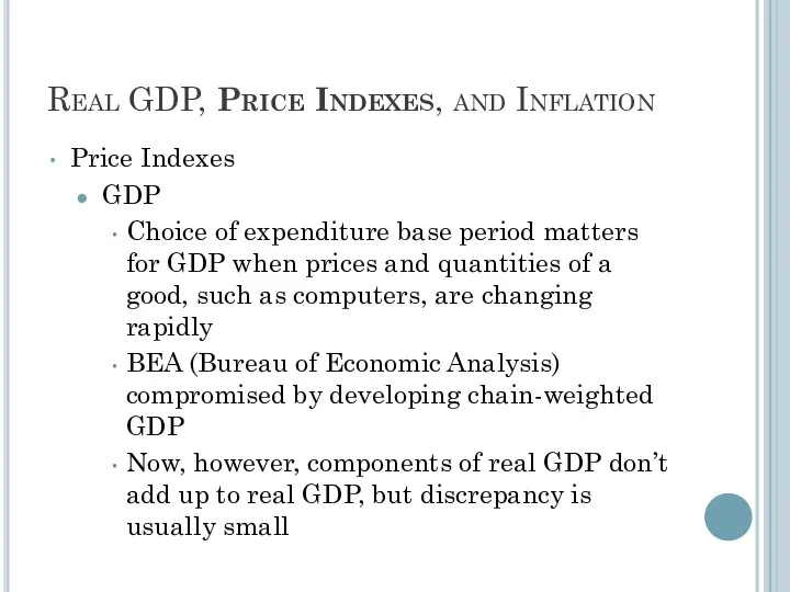
GDP
Choice of expenditure base period
Real GDP, Price Indexes, and Inflation
Price Indexes
GDP
Choice of expenditure base period
Real GDP, Price Indexes, and Inflation
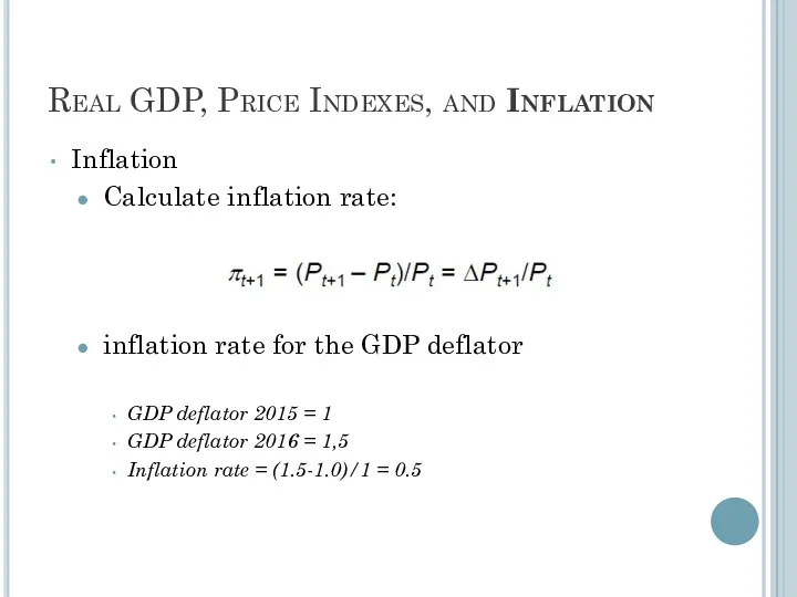
Inflation
Calculate inflation rate:
inflation rate for the
Real GDP, Price Indexes, and Inflation
Inflation
Calculate inflation rate:
inflation rate for the
Real GDP, Price Indexes, and Inflation
Price Indexes
Does CPI inflation overstate increases
Real GDP, Price Indexes, and Inflation
Price Indexes
Does CPI inflation overstate increases
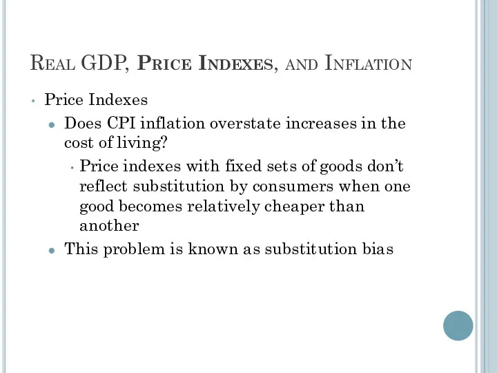
Real GDP, Price Indexes, and Inflation
Price Indexes
Does CPI inflation overstate increases
Real GDP, Price Indexes, and Inflation
Price Indexes
Does CPI inflation overstate increases
Real GDP, Price Indexes, and Inflation
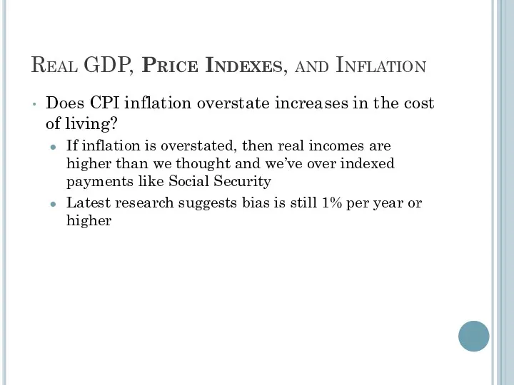
Does CPI inflation overstate increases in
Real GDP, Price Indexes, and Inflation
Does CPI inflation overstate increases in
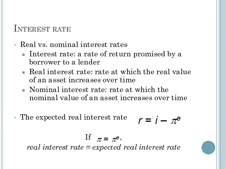
Interest rate
Real vs. nominal interest rates
Interest rate: a rate of return
Interest rate
Real vs. nominal interest rates
Interest rate: a rate of return
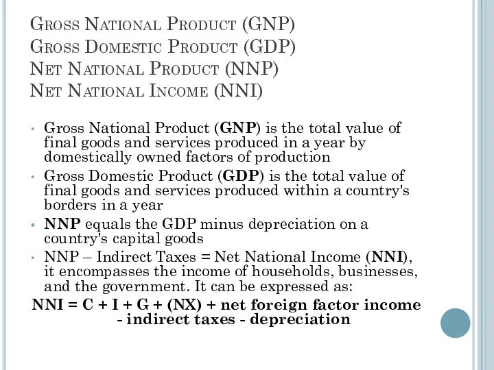
Gross National Product (GNP)
Gross Domestic Product (GDP)
Net National Product (NNP)
Net National
Gross National Product (GNP) Gross Domestic Product (GDP) Net National Product (NNP) Net National
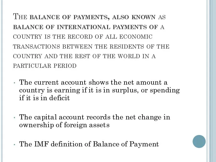
The balance of payments, also known as balance of international payments
The balance of payments, also known as balance of international payments
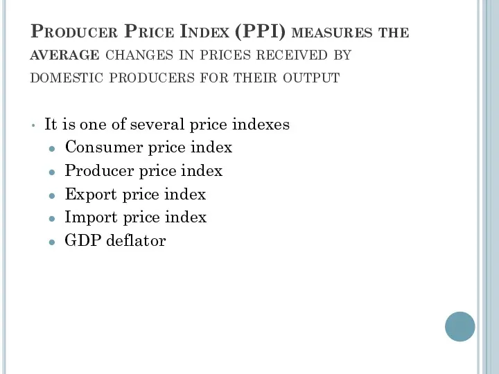
Producer Price Index (PPI) measures the average changes in prices received
Producer Price Index (PPI) measures the average changes in prices received

Macroeconomics
The Measurement and
Structure of the
National Economy
Zharova Liubov
Zharova_l@ua.fm
Macroeconomics
The Measurement and
Structure of the
National Economy
Zharova Liubov
Zharova_l@ua.fm
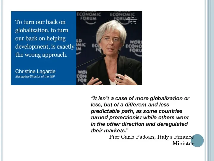
“It isn’t a case of more globalization or less, but of
“It isn’t a case of more globalization or less, but of
What Is Globalization
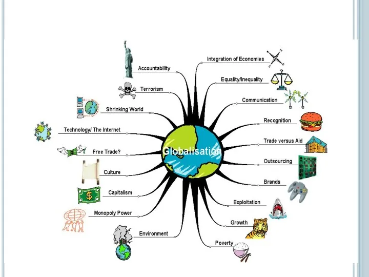
Globalization is defined as a process that, based on
What Is Globalization
Globalization is defined as a process that, based on
basic aspects of globalization
In 2000, the International Monetary Fund (IMF) identified
basic aspects of globalization
In 2000, the International Monetary Fund (IMF) identified
Globalization Encompasses
Internationalization (trade & investment)
Liberalization (freeing markets)
Universalization (cultural interchange)…or…
Westernization (Western cultural
Globalization Encompasses
Internationalization (trade & investment)
Liberalization (freeing markets)
Universalization (cultural interchange)…or…
Westernization (Western cultural
Impact
Economic impact
Improvement in standard of living
Increased competition among nations
Widening income gap
Impact
Economic impact
Improvement in standard of living
Increased competition among nations
Widening income gap
Focus on: Measuring globalisation
STATISTICAL INDICATORS
OECD Economic Globalization Indicators helps identify the
Focus on: Measuring globalisation
STATISTICAL INDICATORS
OECD Economic Globalization Indicators helps identify the
Focus on: Measuring globalisation
STATISTICAL INDICATORS
UNCTAD Development and Globalization: Facts and
Focus on: Measuring globalisation
STATISTICAL INDICATORS
UNCTAD Development and Globalization: Facts and
Focus on: Measuring globalisation
COMPOSITE INDEXES
The A. T Kearney/FOREIGN POLICY Globalization Index
Focus on: Measuring globalisation
COMPOSITE INDEXES
The A. T Kearney/FOREIGN POLICY Globalization Index
The A. T Kearney/FOREIGN POLICY Globalization Index (Ukraine 39)
The A. T Kearney/FOREIGN POLICY Globalization Index (Ukraine 39)
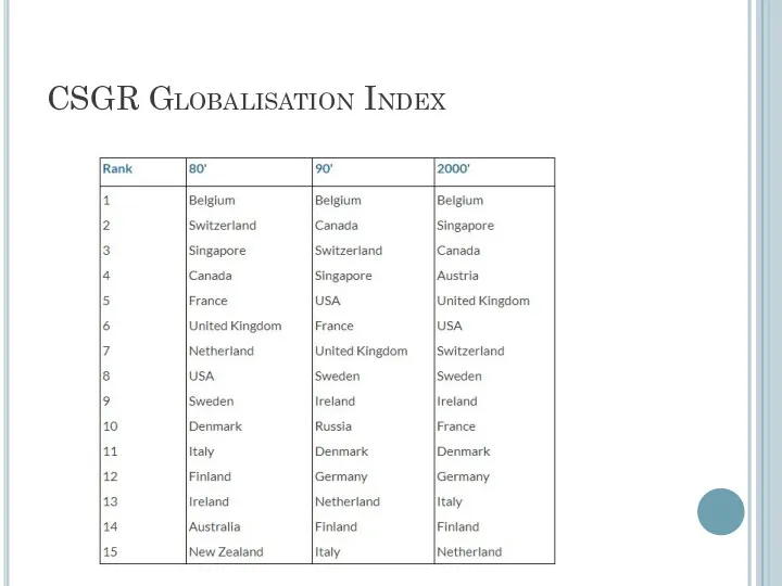
CSGR Globalisation Index
CSGR Globalisation Index
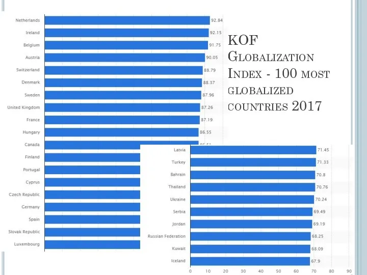
KOF Globalization Index - 100 most globalized countries 2017
KOF Globalization Index - 100 most globalized countries 2017
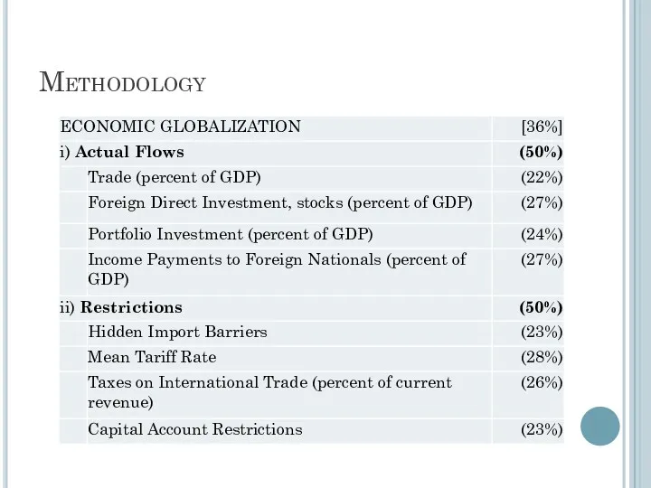
Methodology
Methodology
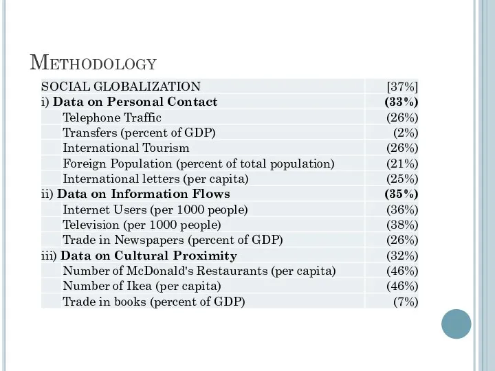
Methodology
Methodology
![Methodology POLITICAL GLOBALIZATION [27%] Embassies in Country (25%) Membership in](/_ipx/f_webp&q_80&fit_contain&s_1440x1080/imagesDir/jpg/304152/slide-129.jpg)
Methodology
POLITICAL GLOBALIZATION [27%]
Embassies in Country (25%)
Membership in International Organizations (27%)
Participation in U.N. Security Council
Methodology
POLITICAL GLOBALIZATION [27%]
Embassies in Country (25%)
Membership in International Organizations (27%)
Participation in U.N. Security Council

“Arguably no other place on earth has so engineered itself to
“Arguably no other place on earth has so engineered itself to
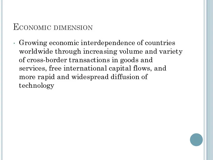
Economic dimension
Growing economic interdependence of countries worldwide through increasing volume and
Economic dimension
Growing economic interdependence of countries worldwide through increasing volume and
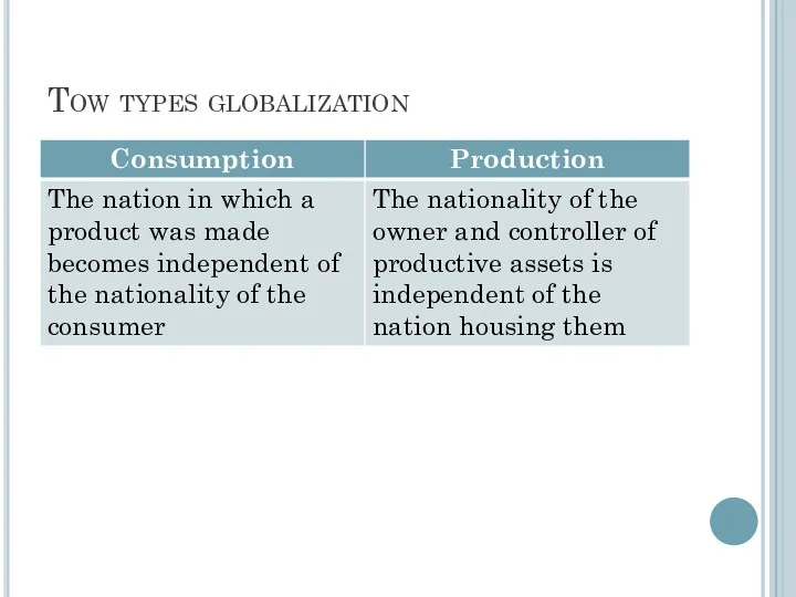
Tow types globalization
Tow types globalization
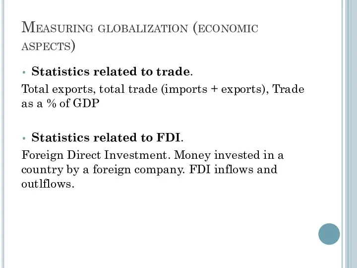
Measuring globalization (economic aspects)
Statistics related to trade.
Total exports, total trade
Measuring globalization (economic aspects)
Statistics related to trade.
Total exports, total trade
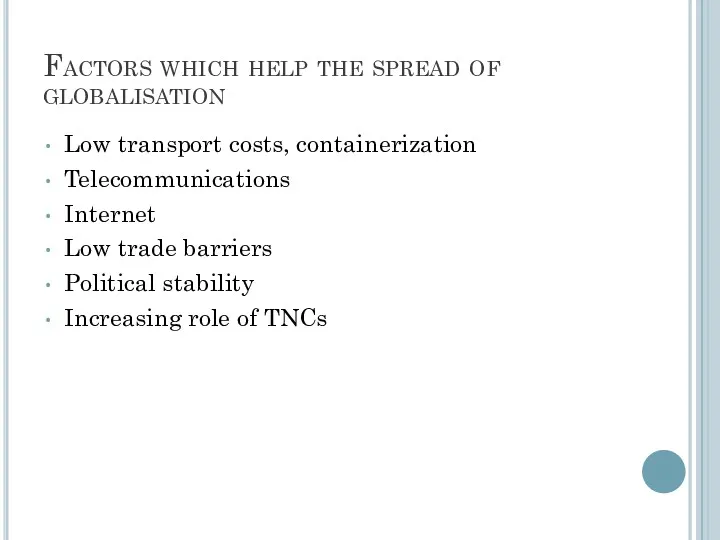
Factors which help the spread of globalisation
Low transport costs, containerization
Telecommunications
Internet
Low
Factors which help the spread of globalisation
Low transport costs, containerization
Telecommunications
Internet
Low
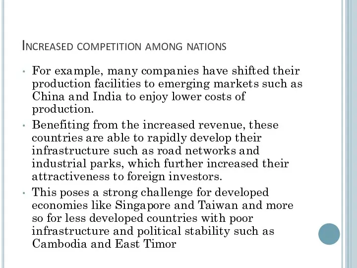
Increased competition among nations
For example, many companies have shifted their production
Increased competition among nations
For example, many companies have shifted their production

Increased competition among nations
“They (economists) predict that increased competition from low-wage
Increased competition among nations
“They (economists) predict that increased competition from low-wage
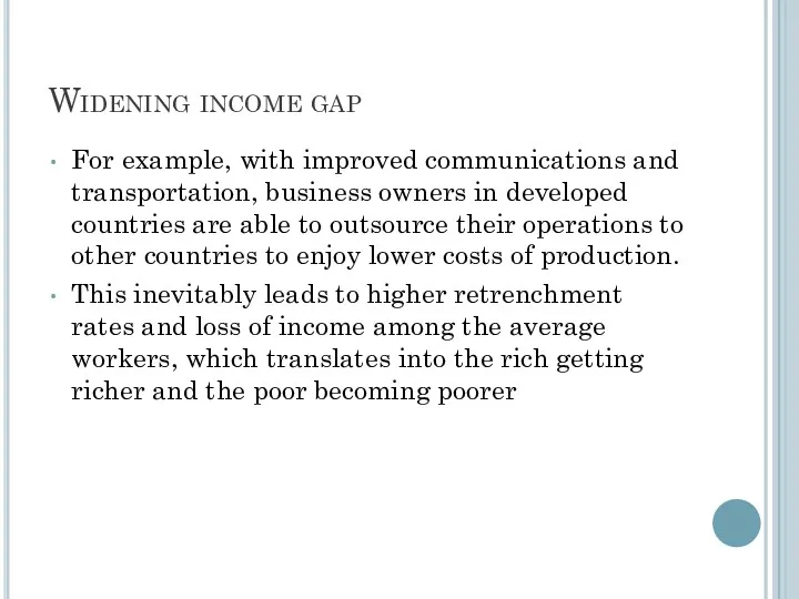
Widening income gap
For example, with improved communications and transportation, business owners
Widening income gap
For example, with improved communications and transportation, business owners
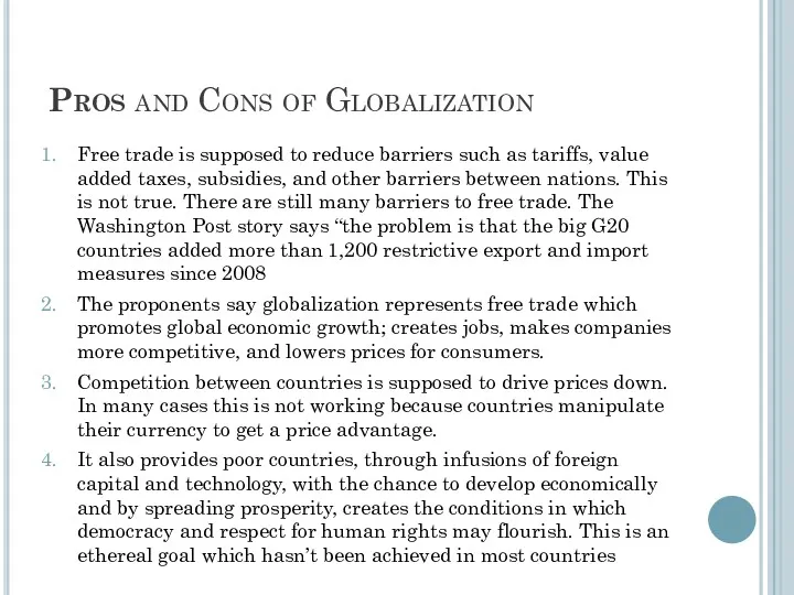
Pros and Cons of Globalization
Free trade is supposed to reduce barriers
Pros and Cons of Globalization
Free trade is supposed to reduce barriers

Pros & Cons
According to supporters globalization and democracy should go hand
Pros & Cons
According to supporters globalization and democracy should go hand
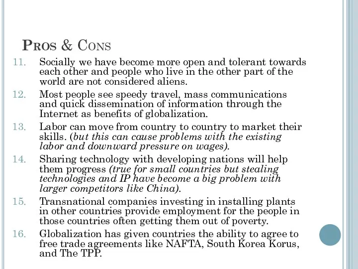
Pros & Cons
Socially we have become more open and tolerant towards
Pros & Cons
Socially we have become more open and tolerant towards
Pros & Cons
The general complaint about globalization is that it has
Pros & Cons
The general complaint about globalization is that it has
Pros & Cons
Workers in developed countries like the US face pay-cut
Pros & Cons
Workers in developed countries like the US face pay-cut
Pros & Cons
The anti-globalists also claim that globalization is not working
Pros & Cons
The anti-globalists also claim that globalization is not working

Documentory
Documentory
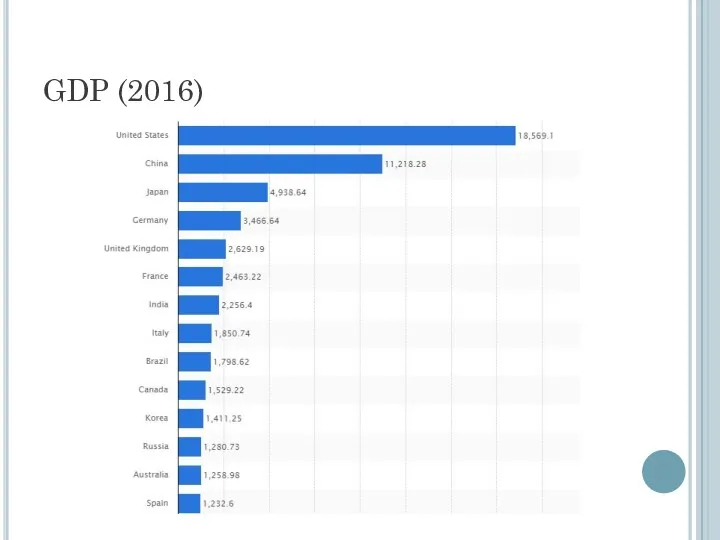
GDP (2016)
GDP (2016)
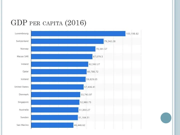
GDP per capita (2016)
GDP per capita (2016)
Macroeconomics
Productivity, Output & Employment
Zharova Liubov
Zharova_l@ua.fm
Macroeconomics
Productivity, Output & Employment
Zharova Liubov
Zharova_l@ua.fm
How much does the economy produce?
The quantity that an economy will
How much does the economy produce?
The quantity that an economy will
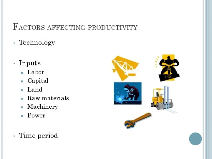
Factors affecting productivity
Technology
Inputs
Labor
Capital
Land
Raw materials
Machinery
Power
Time period
Factors affecting productivity
Technology
Inputs
Labor
Capital
Land
Raw materials
Machinery
Power
Time period
The production function
The quantity of inputs does not completely determine the
The production function
The quantity of inputs does not completely determine the
Empirical example: US production function
Studies show that the relationship between outputs
Empirical example: US production function
Studies show that the relationship between outputs
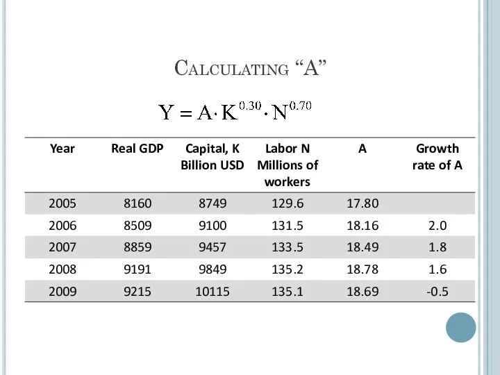
Calculating “A”
Calculating “A”
Shape of the production function
We can have an idea about the
Shape of the production function
We can have an idea about the
Shape of the production function
Shape of the production function
Shape of the production function: Properties
The production function slopes upward from
Shape of the production function: Properties
The production function slopes upward from
Effect of increasing 1000 units of capital each time
Marginal Product of
Effect of increasing 1000 units of capital each time
Marginal Product of
Marginal productivity
The previous example shows that marginal productivity is falling as
Marginal productivity
The previous example shows that marginal productivity is falling as
Formal Definitions of Marginal Productivity
Marginal Productivity of Capital: means additional output
Formal Definitions of Marginal Productivity
Marginal Productivity of Capital: means additional output
Changes in the production function
The production function does not remain fixed
Changes in the production function
The production function does not remain fixed
Demand for labor
In contrast to the amount of capital, the amount
Demand for labor
In contrast to the amount of capital, the amount
Determination of the demand for labor
Demand for labor is determined based
Determination of the demand for labor
Demand for labor is determined based
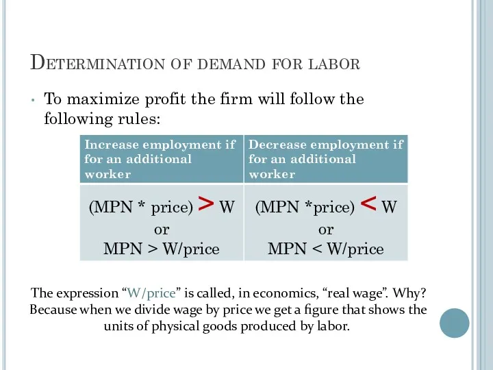
Determination of demand for labor
To maximize profit the firm will follow
Determination of demand for labor
To maximize profit the firm will follow
Determination of labor demand
w*
N*
MPN and real wage
Labor
MPN
Real wage
The MPN curve on
Determination of labor demand
w*
N*
MPN and real wage
Labor
MPN
Real wage
The MPN curve on
Factors that shift labor demand curve
Changes in the wage do not
Factors that shift labor demand curve
Changes in the wage do not
Shift of the labor demand curve
A beneficial supply shock, such as
Shift of the labor demand curve
A beneficial supply shock, such as
Supply of labor
We have seen that firm’s demand for labor depend
Supply of labor
We have seen that firm’s demand for labor depend
Labor supply curve
Labor supply curve looks the same as the supply
Labor supply curve
Labor supply curve looks the same as the supply
Factors that shift the labor supply curve
Left
Left
Right
Right
Factors that shift the labor supply curve
Left
Left
Right
Right
Labor market equilibrium
w*
MPN and real wage
labor
MPN/demand for labor
Real wage
A
Labor supply
Labor market equilibrium
w*
MPN and real wage
labor
MPN/demand for labor
Real wage
A
Labor supply
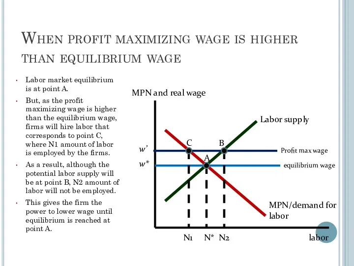
When profit maximizing wage is higher than equilibrium wage
Labor market equilibrium
When profit maximizing wage is higher than equilibrium wage
Labor market equilibrium
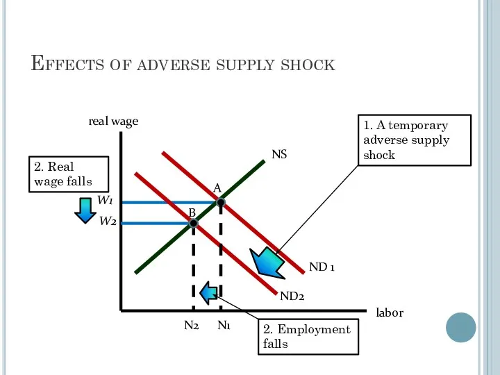
Effects of adverse supply shock
W2
N2
real wage
labor
ND 1
B
N1
ND2
A
W1
NS
1. A temporary adverse supply
Effects of adverse supply shock
W2
N2
real wage
labor
ND 1
B
N1
ND2
A
W1
NS
1. A temporary adverse supply
What if all workers are not alike?
We assumed that all workers
What if all workers are not alike?
We assumed that all workers
Unemployment: the untold story of full-employment
Full-employment level implies that all the
Unemployment: the untold story of full-employment
Full-employment level implies that all the

Productivity / GDP per capita & GDP (PPP)
Prof. Zharova Liubov
Zharova_l@ua.fm
Productivity / GDP per capita & GDP (PPP)
Prof. Zharova Liubov
Zharova_l@ua.fm
GDP Per Capita / GDP PPP (purchasing parity power)
GDP per
GDP Per Capita / GDP PPP (purchasing parity power)
GDP per
Why do we need GDP per capita?
sometimes used as an indicator
Why do we need GDP per capita?
sometimes used as an indicator
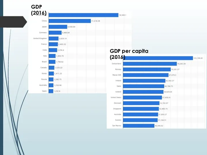
GDP (2016)
GDP per capita (2016)
GDP (2016)
GDP per capita (2016)
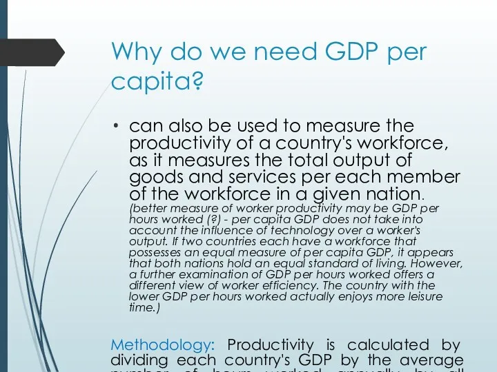
Why do we need GDP per capita?
can also be used to
Why do we need GDP per capita?
can also be used to
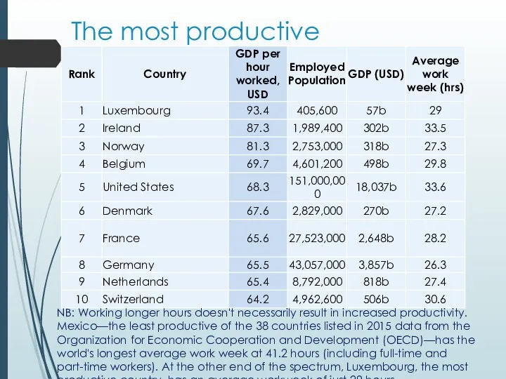
The most productive countries (2015)
NB: Working longer hours doesn't necessarily result
The most productive countries (2015)
NB: Working longer hours doesn't necessarily result
Labour productivity
Labour productivity is defined as real gross domestic product (GDP)
Labour productivity
Labour productivity is defined as real gross domestic product (GDP)
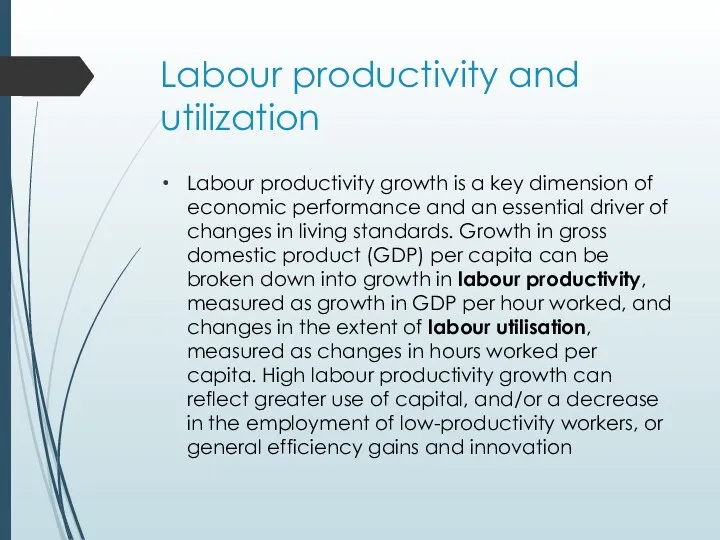
Labour productivity and utilization
Labour productivity growth is a key dimension of
Labour productivity and utilization
Labour productivity growth is a key dimension of
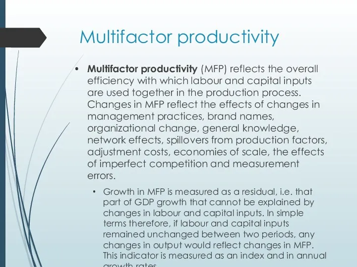
Multifactor productivity
Multifactor productivity (MFP) reflects the overall efficiency with which labour
Multifactor productivity
Multifactor productivity (MFP) reflects the overall efficiency with which labour
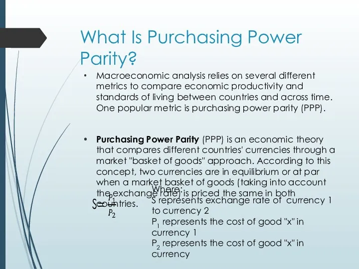
What Is Purchasing Power Parity?
Macroeconomic analysis relies on several different metrics
What Is Purchasing Power Parity?
Macroeconomic analysis relies on several different metrics
PPP calculation
Problem: To make a comparison of prices across countries that
PPP calculation
Problem: To make a comparison of prices across countries that
The Big Mac Index: an example of PPP
(The Economist)
Prehistory: The Economist
The Big Mac Index: an example of PPP
(The Economist)
Prehistory: The Economist
GDP with PPP
Example: One way to think of what GDP with
GDP with PPP
Example: One way to think of what GDP with
Transport Costs: Goods that are not available locally will need to
Transport Costs: Goods that are not available locally will need to

Venezuela case
Venezuela case
From the 10 years of military dictatorship between 1948-1958 to the
From the 10 years of military dictatorship between 1948-1958 to the
By 1950, as the rest of the world was struggling to
By 1950, as the rest of the world was struggling to
The Downfall of Venezuela’s Economy
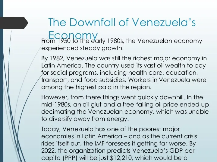
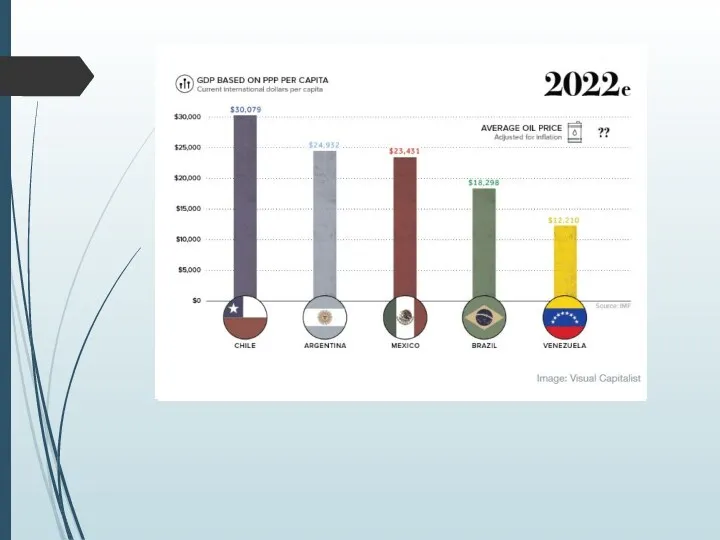
From 1950 to the early 1980s, the
The Downfall of Venezuela’s Economy
From 1950 to the early 1980s, the
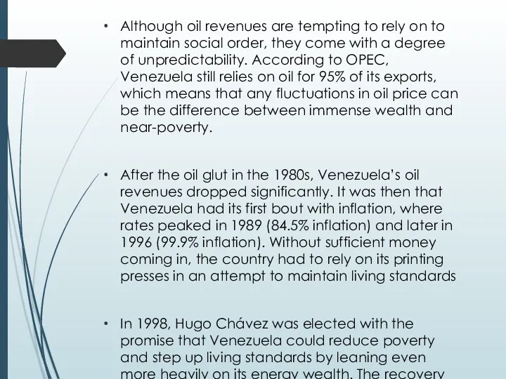
Although oil revenues are tempting to rely on to maintain social
Although oil revenues are tempting to rely on to maintain social
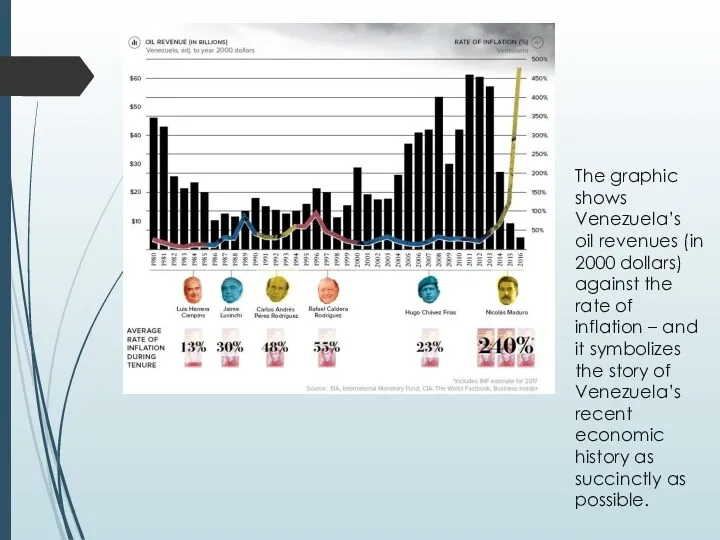
The graphic shows Venezuela’s oil revenues (in 2000 dollars) against the
The graphic shows Venezuela’s oil revenues (in 2000 dollars) against the
Nicolás Maduro, who took over after the death of his predecessor,
Nicolás Maduro, who took over after the death of his predecessor,
The details of today’s crisis and intense hyperinflation are widely shared.
The details of today’s crisis and intense hyperinflation are widely shared.
Macroeconomics
Consumption, Savings & Investment
Zharova Liubov
Zharova_l@ua.fm
Macroeconomics
Consumption, Savings & Investment
Zharova Liubov
Zharova_l@ua.fm
Consumption
Consumption can be defined in different ways, but is usually best
Consumption
Consumption can be defined in different ways, but is usually best
Theories of Consumption
Keynes mentioned several subjective and objective factors which determine
Theories of Consumption
Keynes mentioned several subjective and objective factors which determine
S. Kuznets vision
Contrary to Keynes’s proposition that proportion of income
S. Kuznets vision
Contrary to Keynes’s proposition that proportion of income
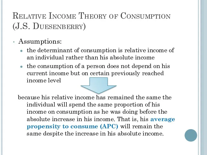
Relative Income Theory of Consumption (J.S. Duesenberry)
Assumptions:
the determinant of consumption
Relative Income Theory of Consumption (J.S. Duesenberry)
Assumptions:
the determinant of consumption
Demonstration Effect: individuals or households try to imitate or copy the
Demonstration Effect: individuals or households try to imitate or copy the
Ratchet Effect - when income of individuals or households falls, their
Ratchet Effect - when income of individuals or households falls, their
Life Cycle Theory of Consumption ( Albert Ando & Franco Modigliani)
Idea: the consumption in any
Life Cycle Theory of Consumption ( Albert Ando & Franco Modigliani)
Idea: the consumption in any
A typical individual in this theory in his early years of
A typical individual in this theory in his early years of
Shortcomings:
criticized the assumption of life cycle hypothesis that in making consumption
Shortcomings:
criticized the assumption of life cycle hypothesis that in making consumption
Permanent Income Theory of Consumption (Milton Friedman)
Assumptions:
consumption is determined by
Permanent Income Theory of Consumption (Milton Friedman)
Assumptions:
consumption is determined by
Relationship between Consumption and Permanent Income: Cp = k(i,w,u) ×Yp
Cp –
Relationship between Consumption and Permanent Income: Cp = k(i,w,u) ×Yp
Cp –
In addition to permanent income (Yp), the individual’s income may contain
In addition to permanent income (Yp), the individual’s income may contain
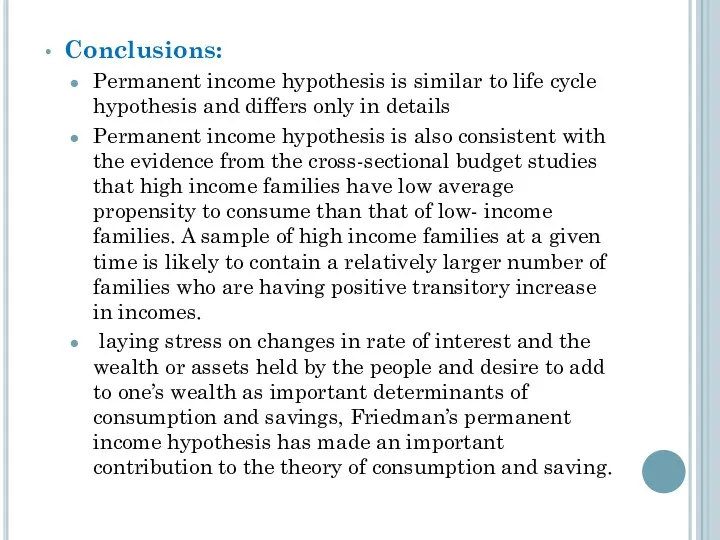
Conclusions:
Permanent income hypothesis is similar to life cycle hypothesis and
Conclusions:
Permanent income hypothesis is similar to life cycle hypothesis and
Real income vs. nominal income
The term 'real' that is used in
Real income vs. nominal income
The term 'real' that is used in
Savings
Savings, according to Keynesian economics, consists of the amount left over when
Savings
Savings, according to Keynesian economics, consists of the amount left over when
Investments
Definition: Money committed or property acquired for future income.
“INVESTMENT” to mean
Investments
Definition: Money committed or property acquired for future income.
“INVESTMENT” to mean
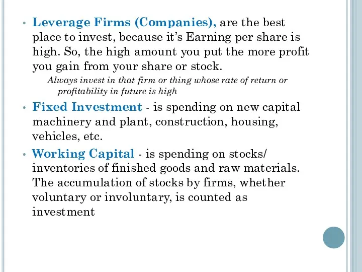
Leverage Firms (Companies), are the best place to invest, because it’s
Leverage Firms (Companies), are the best place to invest, because it’s
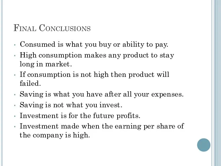
Final Conclusions
Consumed is what you buy or ability to pay.
High consumption
Final Conclusions
Consumed is what you buy or ability to pay.
High consumption
Macroeconomics
GDP
Income
Economic Growth
Zharova Liubov
Macroeconomics
GDP
Income
Economic Growth
Zharova Liubov
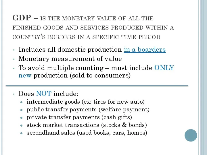
GDP = is the monetary value of all the finished goods
GDP = is the monetary value of all the finished goods
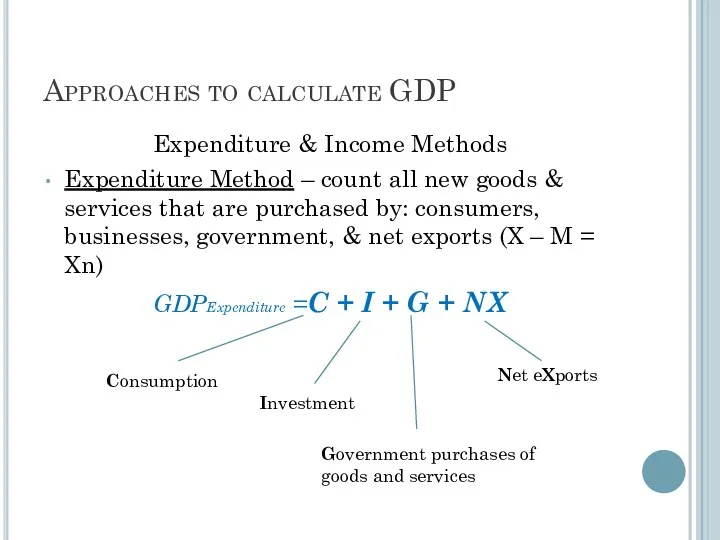
Approaches to calculate GDP
Expenditure & Income Methods
Expenditure Method – count all
Approaches to calculate GDP
Expenditure & Income Methods
Expenditure Method – count all


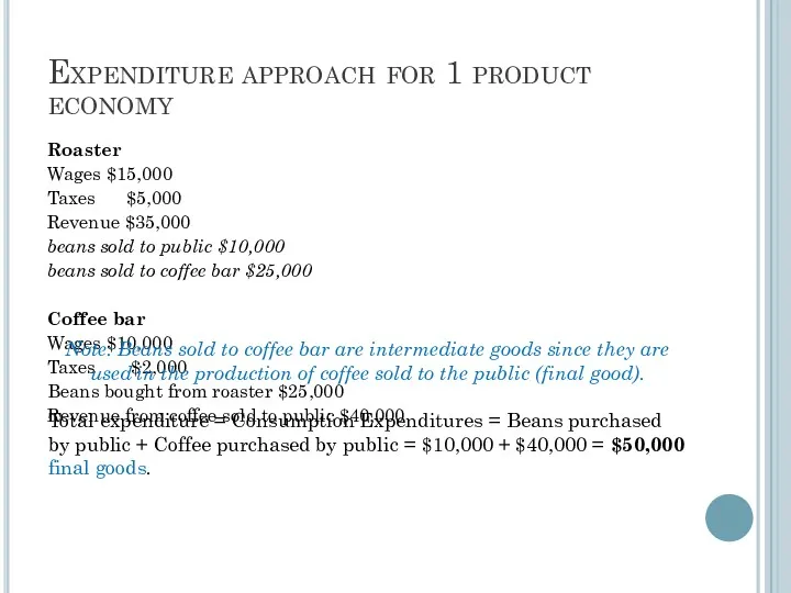
Expenditure approach for 1 product economy
Roaster
Wages $15,000
Taxes $5,000
Revenue $35,000
beans sold to public
Expenditure approach for 1 product economy
Roaster
Wages $15,000
Taxes $5,000
Revenue $35,000
beans sold to public
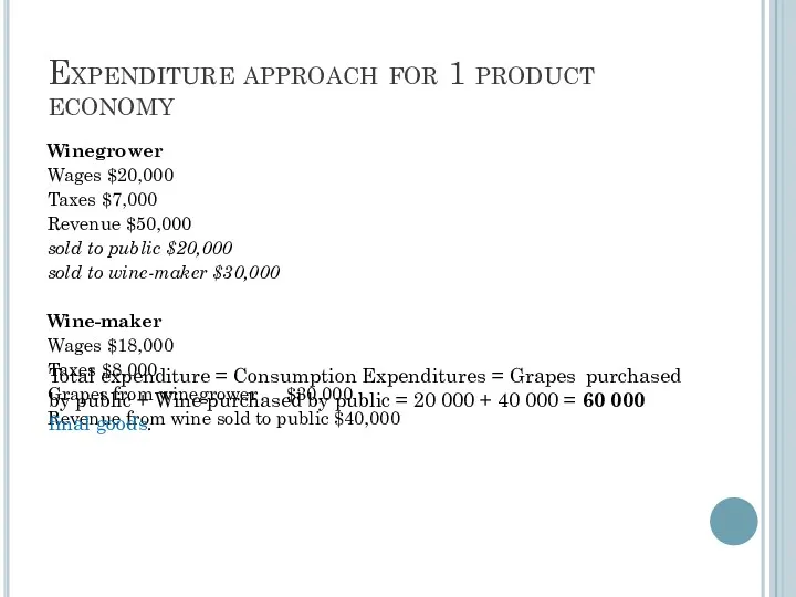
Expenditure approach for 1 product economy
Winegrower
Wages $20,000
Taxes $7,000
Revenue $50,000
sold to public
Expenditure approach for 1 product economy
Winegrower
Wages $20,000
Taxes $7,000
Revenue $50,000
sold to public
Product approach
GDP is the sum of the value added created in
Product approach
GDP is the sum of the value added created in
Product approach for 1 product economy
Roaster
Wages $15,000
Taxes $5,000
Revenue $35,000
beans sold to public
Product approach for 1 product economy
Roaster
Wages $15,000
Taxes $5,000
Revenue $35,000
beans sold to public
Expenditure approach for 1 product economy
Winegrower
Wages $20,000
Taxes $7,000
Revenue $50,000
sold to public
Expenditure approach for 1 product economy
Winegrower
Wages $20,000
Taxes $7,000
Revenue $50,000
sold to public
Income method
Income Method – count all earnings received by those who
Income method
Income Method – count all earnings received by those who
Consumption (C)
Investment (I)
Government purchases (G)
Exports (X)
Imports (M)
Taxes (T)
Saving (S)
(I
Consumption (C)
Investment (I)
Government purchases (G)
Exports (X)
Imports (M)
Taxes (T)
Saving (S)
(I
Consumption
+
Investment
+
Government
+
Net Export
Wages
+
Profits
+
Rents
+
Interest
Depreciation (CCA)
Indirect business taxes (IBT)
GDP in market prices
National income
Expenditure approach
Income
Consumption
+
Investment
+
Government
+
Net Export
Wages
+
Profits
+
Rents
+
Interest
Depreciation (CCA)
Indirect business taxes (IBT)
GDP in market prices
National income
Expenditure approach
Income
NFIA = Factor income earned from abroad by residents - Factor
NFIA = Factor income earned from abroad by residents - Factor
Income approach for 1 product economy
Roaster
Wages $15,000
Taxes $5,000
Revenue $35,000
beans sold to public
Income approach for 1 product economy
Roaster
Wages $15,000
Taxes $5,000
Revenue $35,000
beans sold to public
Income approach for 1 product economy
Winegrower
Wages $20,000
Taxes $7,000
Revenue $50,000
sold to public
Income approach for 1 product economy
Winegrower
Wages $20,000
Taxes $7,000
Revenue $50,000
sold to public
GDP – by sum of Spending, Factor Incomes or Output
GDP – by sum of Spending, Factor Incomes or Output
The first account displays the expenditure and income approaches to measuring
The first account displays the expenditure and income approaches to measuring
GDP (BEA commentaries)
The entries on the right side of account 1
GDP (BEA commentaries)
The entries on the right side of account 1
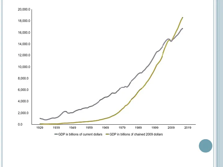
GDP – Nominal vs. Real
Nominal = current year prices
Real = prices
GDP – Nominal vs. Real
Nominal = current year prices
Real = prices
USA GDP Nominal and Real
Real GDP or
GDP in constant prices
USA GDP Nominal and Real
Real GDP or
GDP in constant prices
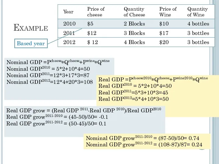
Example
Nominal GDP =Pcheese∗QCheese+Pcheese∗QCheese
Nominal GDP =Pcheese∗Qcheese+Pwine∗Qwine
Nominal GDP2010 = 5*2+10*4=50
Nominal GDP2011=12*3+17*3=87
Nominal GDP2012=12*4+20*3=108
Real
Example
Nominal GDP =Pcheese∗QCheese+Pcheese∗QCheese
Nominal GDP =Pcheese∗Qcheese+Pwine∗Qwine
Nominal GDP2010 = 5*2+10*4=50
Nominal GDP2011=12*3+17*3=87
Nominal GDP2012=12*4+20*3=108
Real
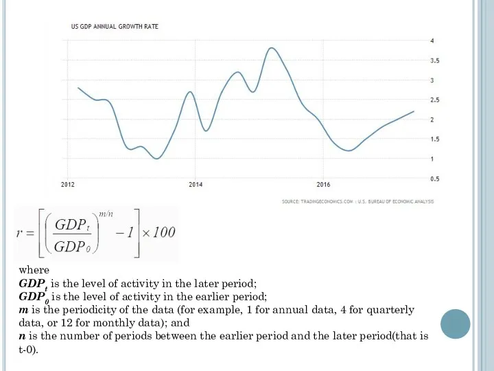
where
GDPt is the level of activity in the later period;
GDP0 is the level
where
GDPt is the level of activity in the later period;
GDP0 is the level
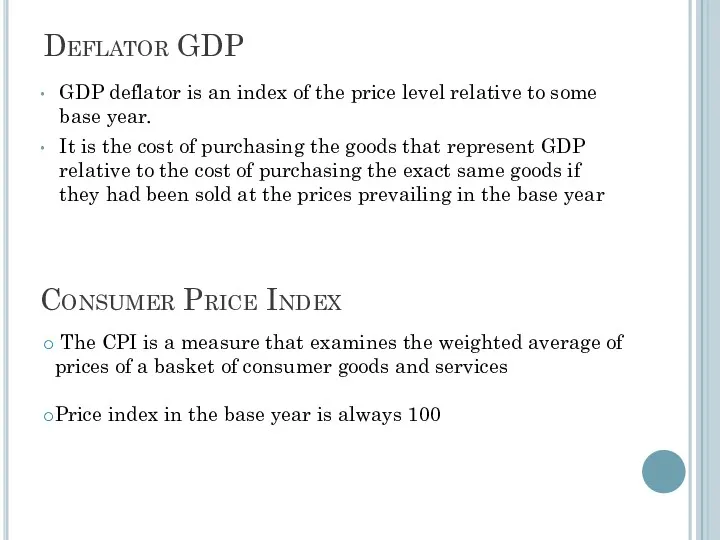
Deflator GDP
GDP deflator is an index of the price level relative
Deflator GDP
GDP deflator is an index of the price level relative
GDP deflator =
Nominal GDP
Real GDP
× 100%
Total amount of money on GDP
GDP deflator =
Nominal GDP
Real GDP
× 100%
Total amount of money on GDP
What is the relationship between GDP deflator & CPI?
Both GDP
What is the relationship between GDP deflator & CPI?
Both GDP
Malaysia
Malaysia
Example
The value of this market basket in the base year :
5
Example
The value of this market basket in the base year :
5
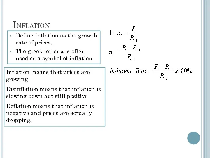
Define Inflation as the growth rate of prices.
The greek letter π
Define Inflation as the growth rate of prices.
The greek letter π
Macroeconomics
GDP /Business Cycle
Unemployment
Zharova Liubov
Macroeconomics
GDP /Business Cycle
Unemployment
Zharova Liubov
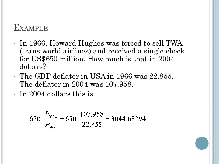
Example
In 1966, Howard Hughes was forced to sell TWA (trans world
Example
In 1966, Howard Hughes was forced to sell TWA (trans world
Trends and cycles
We observe that real GDP is growing over time
Trends and cycles
We observe that real GDP is growing over time
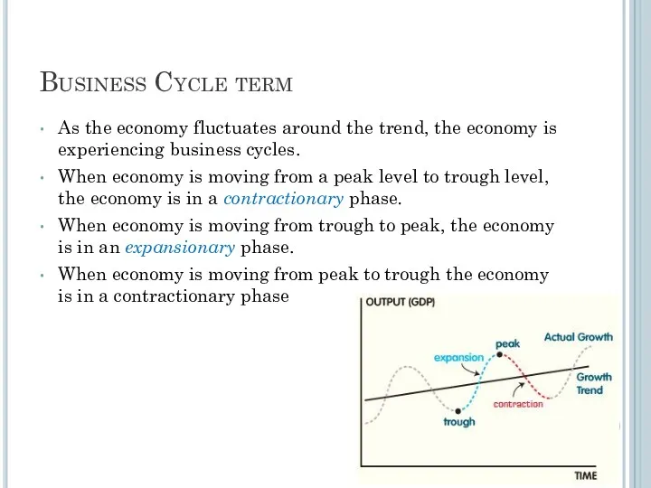
Business Cycle term
As the economy fluctuates around the trend, the economy
Business Cycle term
As the economy fluctuates around the trend, the economy
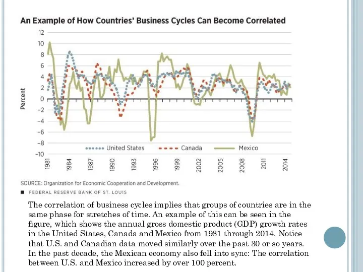
The correlation of business cycles implies that groups of countries are
The correlation of business cycles implies that groups of countries are
North American Free Trade Agreement (NAFTA)
It is a piece of regulation
North American Free Trade Agreement (NAFTA)
It is a piece of regulation
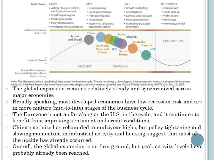
The global expansion remains relatively steady and synchronized across major economies.
Broadly
The global expansion remains relatively steady and synchronized across major economies.
Broadly
Recession and booms
Business cycle positions are sometimes characterized as booms and
Recession and booms
Business cycle positions are sometimes characterized as booms and
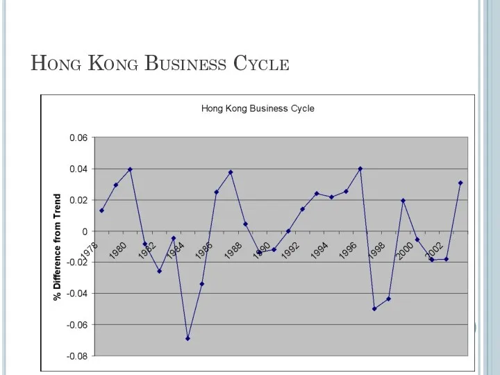
Hong Kong Business Cycle
Hong Kong Business Cycle
Business Cycles & Co-movement
Business cycles are fluctuations in the economy
Business Cycles & Co-movement
Business cycles are fluctuations in the economy
Business Cycles & Sub-Categories
Expenditure. Consumption and Investment co-move with output. Investment
Business Cycles & Sub-Categories
Expenditure. Consumption and Investment co-move with output. Investment
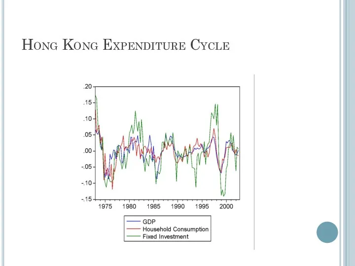
Hong Kong Expenditure Cycle
Hong Kong Expenditure Cycle
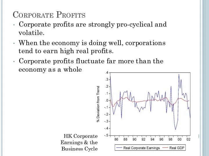
Corporate Profits
Corporate profits are strongly pro-cyclical and volatile.
When the economy is
Corporate Profits
Corporate profits are strongly pro-cyclical and volatile.
When the economy is
Using financial market data to predict business cycles
It has been joked
Using financial market data to predict business cycles
It has been joked
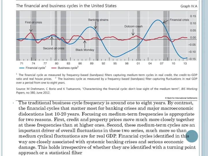
The traditional business cycle frequency is around one to eight years.
The traditional business cycle frequency is around one to eight years.
Level of Unemployment (HK)
Level of Unemployment (HK)
Unemployment
Is defined by the International Labor Organization (ILO) as a situation
Unemployment
Is defined by the International Labor Organization (ILO) as a situation
Unemployment
Labor force
Many people who would like to work but cannot (due
Unemployment
Labor force
Many people who would like to work but cannot (due
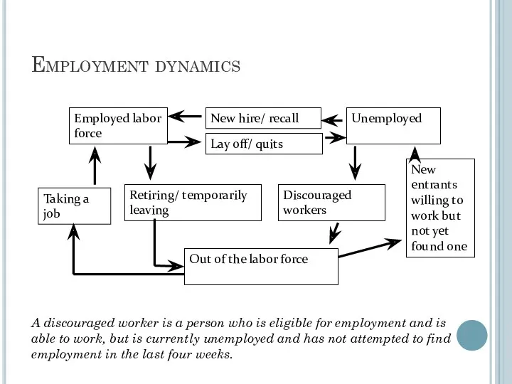
Employment dynamics
Employed labor force
Unemployed
New hire/ recall
Lay off/ quits
Out of the labor
Employment dynamics
Employed labor force
Unemployed
New hire/ recall
Lay off/ quits
Out of the labor
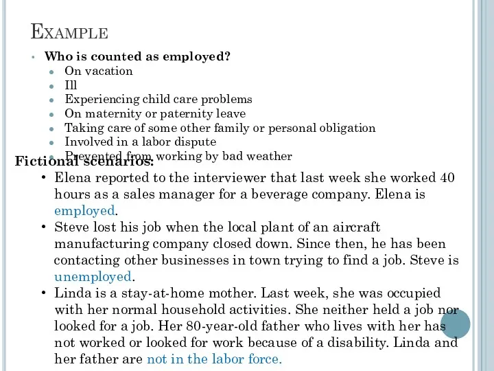
Example
Who is counted as employed?
On vacation
Ill
Experiencing child care problems
On maternity or
Example
Who is counted as employed?
On vacation
Ill
Experiencing child care problems
On maternity or
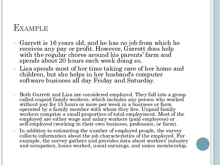
Example
Garrett is 16 years old, and he has no job from
Example
Garrett is 16 years old, and he has no job from
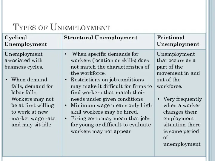
Types of Unemployment
Types of Unemployment
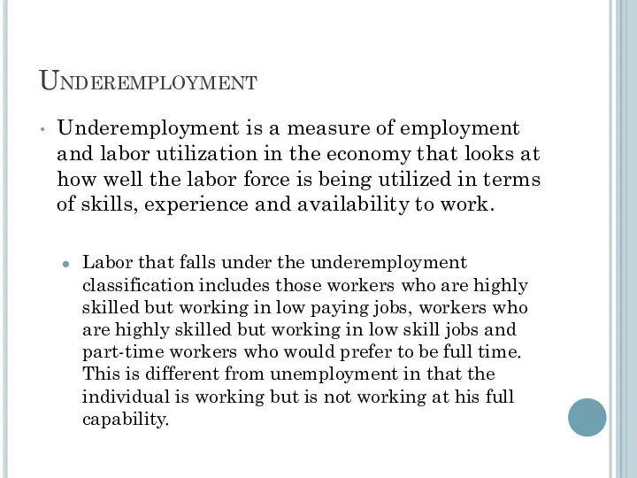
Underemployment
Underemployment is a measure of employment and labor utilization in the
Underemployment
Underemployment is a measure of employment and labor utilization in the
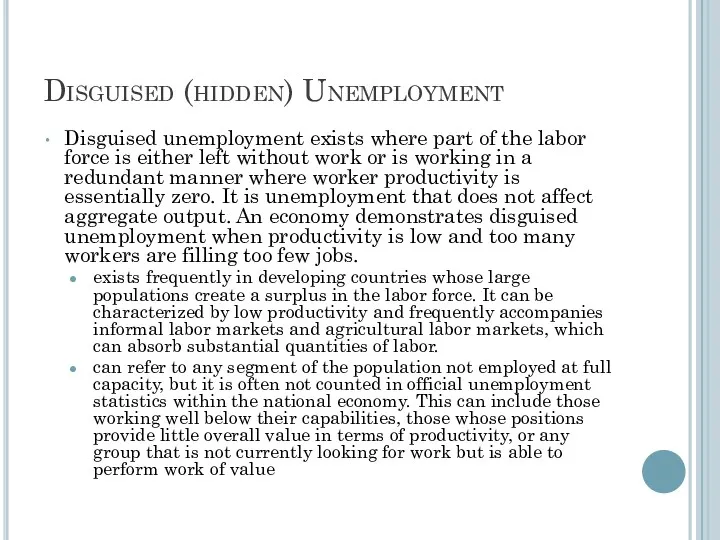
Disguised (hidden) Unemployment
Disguised unemployment exists where part of the labor force
Disguised (hidden) Unemployment
Disguised unemployment exists where part of the labor force
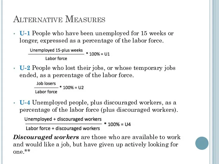
Alternative Measures
U-1 People who have been unemployed for 15 weeks or
Alternative Measures
U-1 People who have been unemployed for 15 weeks or
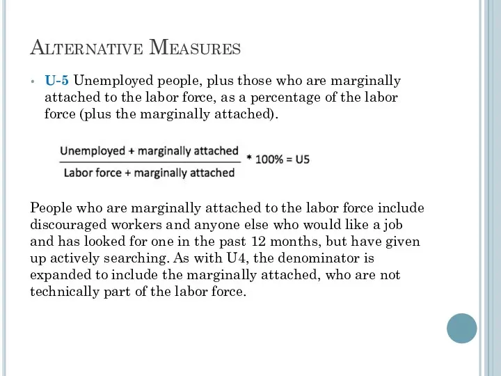
Alternative Measures
U-5 Unemployed people, plus those who are marginally attached to
Alternative Measures
U-5 Unemployed people, plus those who are marginally attached to
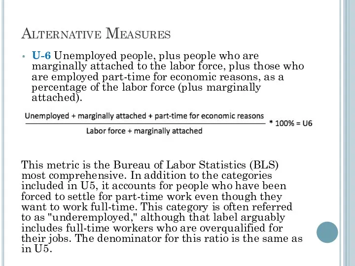
Alternative Measures
U-6 Unemployed people, plus people who are marginally attached to
Alternative Measures
U-6 Unemployed people, plus people who are marginally attached to
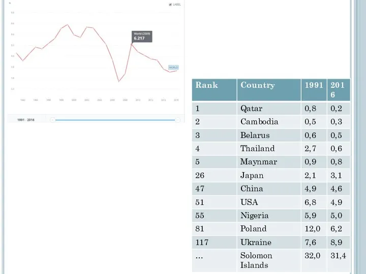
Tightly regulated labor markets increase structural unemployment.
High social welfare benefits increase
Tightly regulated labor markets increase structural unemployment.
High social welfare benefits increase
How to solve the problem
There are two ways the government can
How to solve the problem
There are two ways the government can
Macroeconomics
aggregated supply and demand
Zharova Liubov
Macroeconomics
aggregated supply and demand
Zharova Liubov
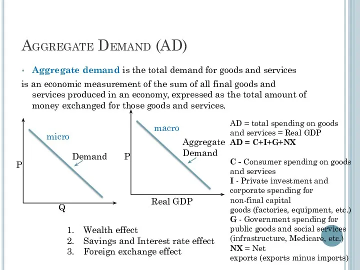
Aggregate Demand (AD)
Aggregate demand is the total demand for goods and
Aggregate Demand (AD)
Aggregate demand is the total demand for goods and
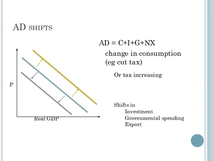
AD shifts
AD = C+I+G+NX
change in consumption (eg cut tax)
Or tax increasing
AD shifts
AD = C+I+G+NX
change in consumption (eg cut tax)
Or tax increasing
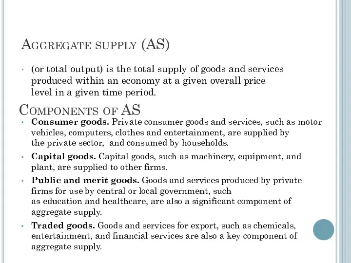
Components of AS
Consumer goods. Private consumer goods and services, such as motor
Components of AS
Consumer goods. Private consumer goods and services, such as motor
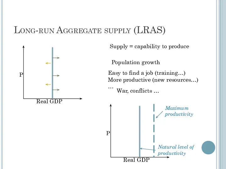
Long-run Aggregate supply (LRAS)
Supply = capability to produce
Population growth
Easy to find
Long-run Aggregate supply (LRAS)
Supply = capability to produce
Population growth
Easy to find
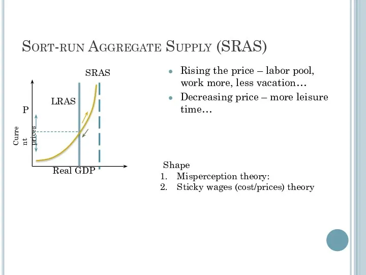
Sort-run Aggregate Supply (SRAS)
Rising the price – labor pool, work more,
Sort-run Aggregate Supply (SRAS)
Rising the price – labor pool, work more,
Summirising
Aggregate supply is the total quantity of output firms will produce and
Summirising
Aggregate supply is the total quantity of output firms will produce and
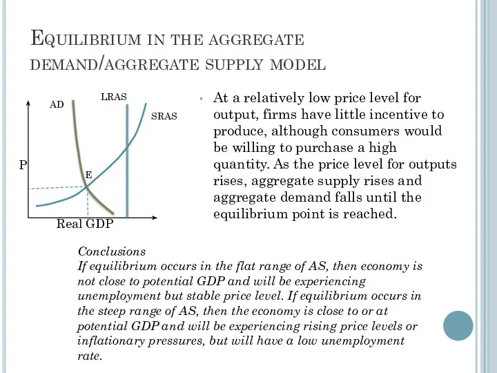
Equilibrium in the aggregate demand/aggregate supply model
At a relatively low price
Equilibrium in the aggregate demand/aggregate supply model
At a relatively low price
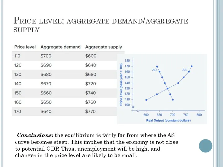
Price level: aggregate demand/aggregate supply
Conclusions: the equilibrium is fairly far from
Price level: aggregate demand/aggregate supply
Conclusions: the equilibrium is fairly far from
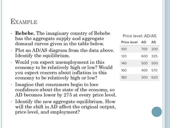
Example
Bebebe. The imaginary country of Bebebe has the aggregate supply and
Example
Bebebe. The imaginary country of Bebebe has the aggregate supply and
How productivity growth shifts the AS curve
Over time, productivity grows so
How productivity growth shifts the AS curve
Over time, productivity grows so
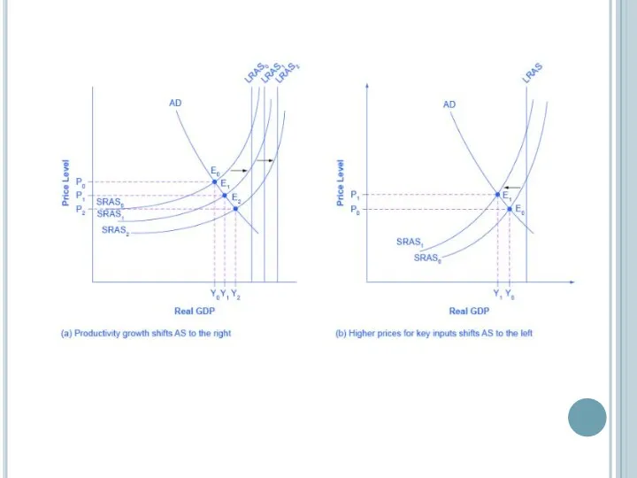
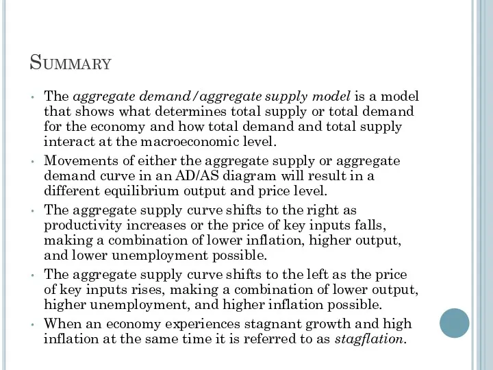
Summary
The aggregate demand/aggregate supply model is a model that shows what determines total
Summary
The aggregate demand/aggregate supply model is a model that shows what determines total
How do changes by consumers and firms affect AD?
When consumers feel
How do changes by consumers and firms affect AD?
When consumers feel
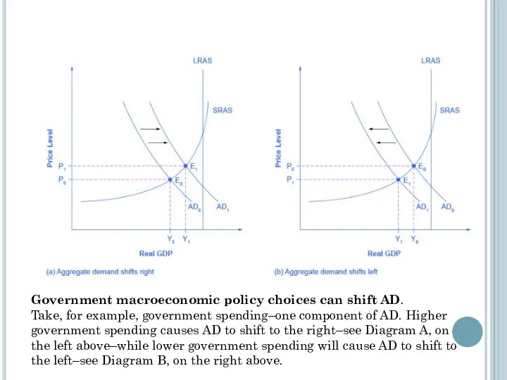
Government macroeconomic policy choices can shift AD.
Take, for example, government spending–one
Government macroeconomic policy choices can shift AD.
Take, for example, government spending–one
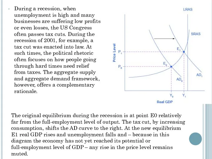
During a recession, when unemployment is high and many businesses are
During a recession, when unemployment is high and many businesses are
 Производительность труда и поддержка занятости
 Экономическое развитие и инновационная экономика
 Економіка і соціологія праці
 Види економічного аналізу. Організація аналізу господарської діяльності. Тема №3
 Применение механизма энергосервисного контракта при переводе автомобильного транспорта на газ - планы и перспективы
 Теория экономического анализа
 Теоретические основы государственного и муниципального сектора
 Национальная экономика как система
 Фонд Сколково. Инновации в ТЭК и предложение по сотрудничеству со странами БРИКС
 Проектная работа. Социально – экономическая статистика
 На пороге нового века: динамика и противоречия экономического развития
 O’zbekistonda tashkil etilgan erkin iqtisodiy zonalarning tashqi savdoni rivojlantirishga ta’siri
 Инфляция: сущность, виды и методы борьбы
 Кругооборот и оборот капитала. Основной и оборотный капитал
 Міжнародна модифікація світового ринку праці
 Анализ и менеджмент экономической деятельности
 Информатизация экономического пространства ЕАЭС
 Презентация Система национальных счетов. Валовой внутренний продукт 11 класс
 Презентация по экономике
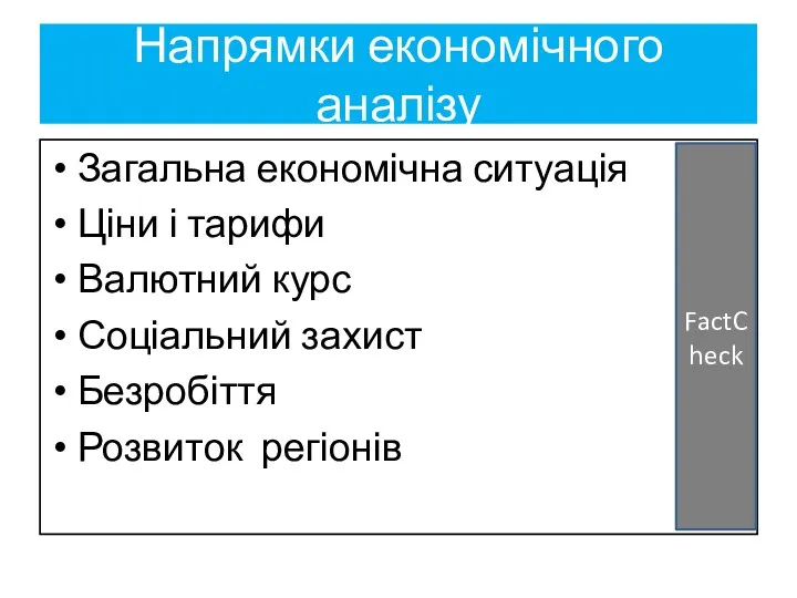 Напрямки економічного аналізу
 Экономика и Государство
 Функционально-стоимостной анализ
 Экономика и государство
 Общая характеристика переходной экономики и ее закономерности
 Капитал как основа предпринимательской деятельности. Лекция 8
 Гравитационная модель и социально-экономическое развитие Курской области и Черноземья
 Концептуальные подходы к управлению проектными рисками в нефтегазовой отрасли
 Өнеркәсіп географиясы