- Business Cycle Theory: The Economy in the Short Run

Содержание
- 2. INTRODUCTION TO ECONOMIC FLUCTUATIONS 10
- 3. 10-1 The Facts About the Business Cycle 10-2 Time Horizons in Macroeconomics 10-3 Aggregate Demand 10-4
- 4. When the economy experiences a period of falling output and rising unemployment, the economy is said
- 5. Real GDP Growth in the United States Growth in real GDP averages about 3% per year,
- 6. Growth in Consumption and Investment When the economy heads into a RECESSION, growth in real consumption
- 7. Unemployment The U rises significantly during periods of recession, shown here by the shaded areas.
- 8. Okun’s Law This figure is a scatter plot of the change in the UR on the
- 9. What relationship should we expect between U and real GDP? Unemployed workers do not help to
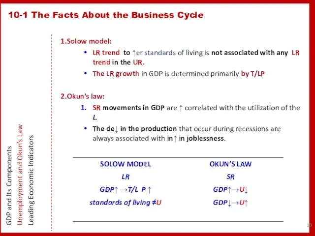
- 10. 10-1 The Facts About the Business Cycle GDP and Its Components Unemployment and Okun’s Law Leading
- 11. Economists arrive at their forecasts is by looking at leading indicators, which are variables that tend
- 12. Average WORKWEEK of production workers in manufacturing. A shorter workweek => lay off workers cut back
- 13. The theoretical separation of real and nominal variables is called the classical dichotomy. The irrelevance of
- 14. 2 If You Want to Know Why Firms Have Sticky Prices, Ask Them
- 16. How does the introduction of StP change our view of how the economy works? By S&D:
- 17. 10-2 Time Horizons in Macroeconomics How the Short Run and Long Run Differ The Model of
- 18. Aggregate demand (AD) is the relationship between the quantity of Y demanded and the aggregate P.
- 19. 10-3 Aggregate Demand The Quantity Equation as Aggregate Demand Why the Aggregate Demand Curve Slopes Downward
- 20. 10-3 Aggregate Demand The Quantity Equation as Aggregate Demand Why the Aggregate Demand Curve Slopes Downward
- 21. 10-3 Aggregate Demand The Quantity Equation as Aggregate Demand Why the Aggregate Demand Curve Slopes Downward
- 22. 10-3 Aggregate Demand The Quantity Equation as Aggregate Demand Why the Aggregate Demand Curve Slopes Downward
- 23. Shifts in the Aggregate Demand Curve Changes in the M shift the AD curve. In panel
- 24. 10-4 Aggregate Supply The Long Run: The Vertical Aggregate Supply Curve The Short Run: The Horizontal
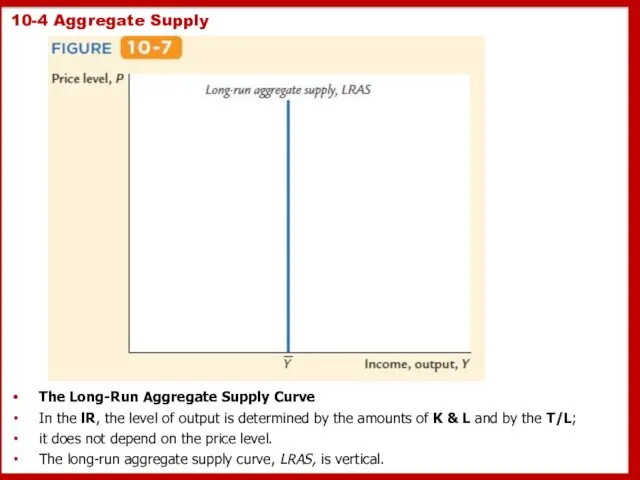
- 25. 10-4 Aggregate Supply The Long-Run Aggregate Supply Curve In the lR, the level of output is
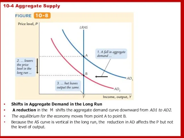
- 26. 10-4 Aggregate Supply Shifts in Aggregate Demand in the Long Run A reduction in the M
- 27. 10-4 Aggregate Supply The Short-Run Aggregate Supply Curve In this extreme example, all prices are fixed
- 28. 10-4 Aggregate Supply Shifts in Aggregate Demand in the Short Run A reduction in the M
- 29. 10-4 Aggregate Supply Long-Run Equilibrium In the LR, the economy finds itself at the intersection of
- 30. 10-4 Aggregate Supply A Reduction in Aggregate Demand The economy begins in long-run equilibrium at point
- 31. The story begins with the unusual nature of French money at the time. The money stock
- 32. Here is how Hume described a monetary injection in his 1752 essay Of Money: To account,
- 33. Fluctuations in the economy as a whole come from changes AS or AD. Economists call exogenous
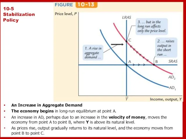
- 34. 10-5 Stabilization Policy An Increase in Aggregate Demand The economy begins in long-run equilibrium at point
- 35. Because supply shocks have a direct impact on the price level, they are sometimes called price
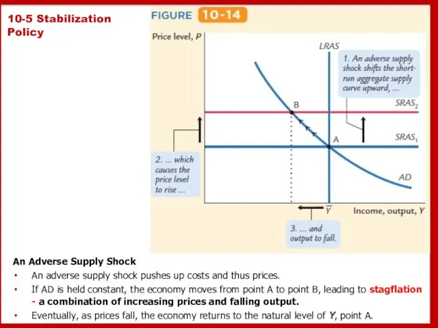
- 36. 10-5 Stabilization Policy An Adverse Supply Shock An adverse supply shock pushes up costs and thus
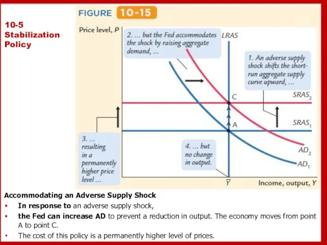
- 37. 10-5 Stabilization Policy Accommodating an Adverse Supply Shock In response to an adverse supply shock, the
- 38. How OPEC Helped Cause Stagflation in the 1970s and Euphoria in the 1980s
- 39. 10-6 Conclusion This chapter introduced a framework to study economic fluctuations: the model of aggregate supply
- 41. Скачать презентацию
INTRODUCTION TO ECONOMIC FLUCTUATIONS
10
INTRODUCTION TO ECONOMIC FLUCTUATIONS
10
10-1 The Facts About the Business Cycle
10-2 Time Horizons in Macroeconomics
10-3
10-1 The Facts About the Business Cycle
10-2 Time Horizons in Macroeconomics
10-3
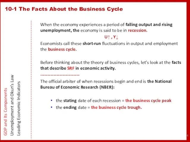
When the economy experiences a period of falling output and rising
When the economy experiences a period of falling output and rising
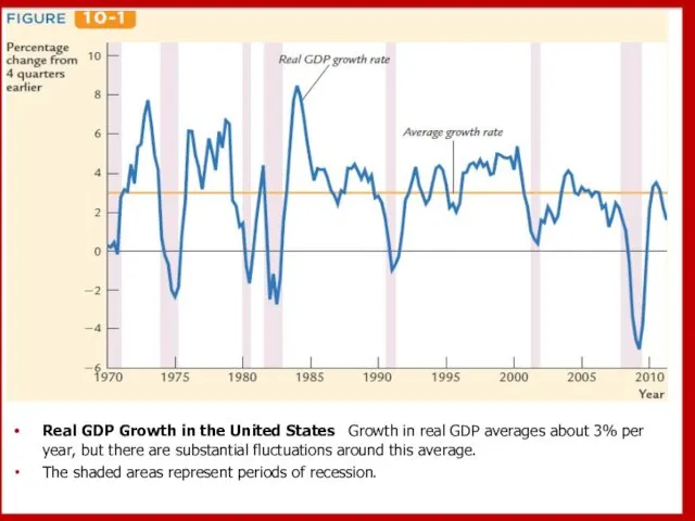
Real GDP Growth in the United States Growth in real GDP
Real GDP Growth in the United States Growth in real GDP
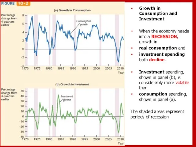
Growth in Consumption and Investment
When the economy heads into a RECESSION,
Growth in Consumption and Investment
When the economy heads into a RECESSION,
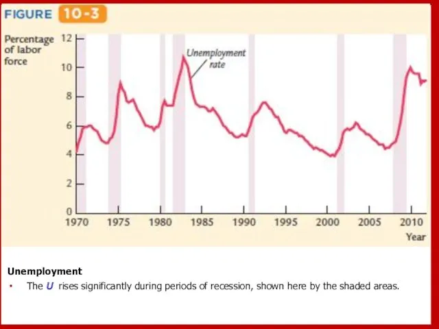
Unemployment
The U rises significantly during periods of recession, shown here
Unemployment
The U rises significantly during periods of recession, shown here
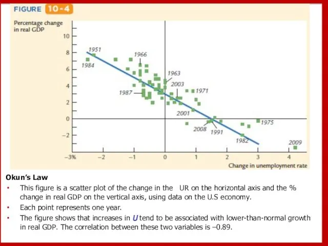
Okun’s Law
This figure is a scatter plot of the change
Okun’s Law
This figure is a scatter plot of the change
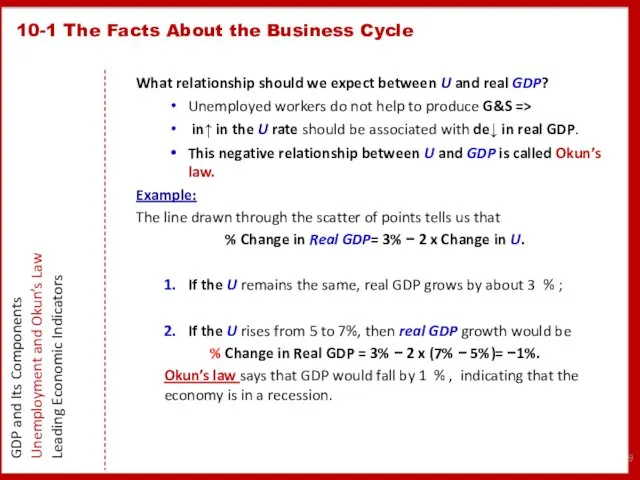
What relationship should we expect between U and real GDP?
Unemployed workers
What relationship should we expect between U and real GDP?
Unemployed workers
10-1 The Facts About the Business Cycle
GDP and Its Components
Unemployment and
10-1 The Facts About the Business Cycle
GDP and Its Components
Unemployment and
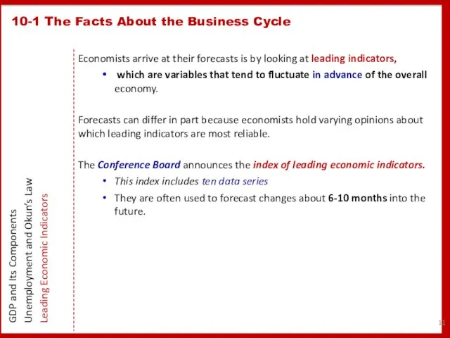
Economists arrive at their forecasts is by looking at leading indicators,
Economists arrive at their forecasts is by looking at leading indicators,
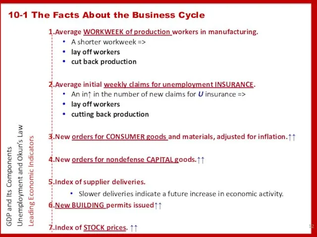
Average WORKWEEK of production workers in manufacturing.
A shorter workweek =>
lay
Average WORKWEEK of production workers in manufacturing.
A shorter workweek =>
lay
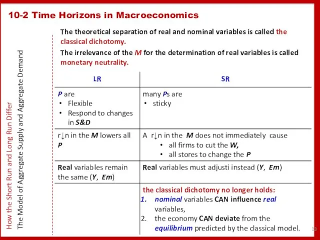
The theoretical separation of real and nominal variables is called the
The theoretical separation of real and nominal variables is called the
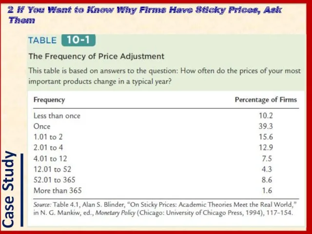
2 If You Want to Know Why Firms Have Sticky Prices,
2 If You Want to Know Why Firms Have Sticky Prices,

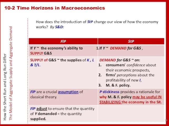
How does the introduction of StP change our view of how
How does the introduction of StP change our view of how
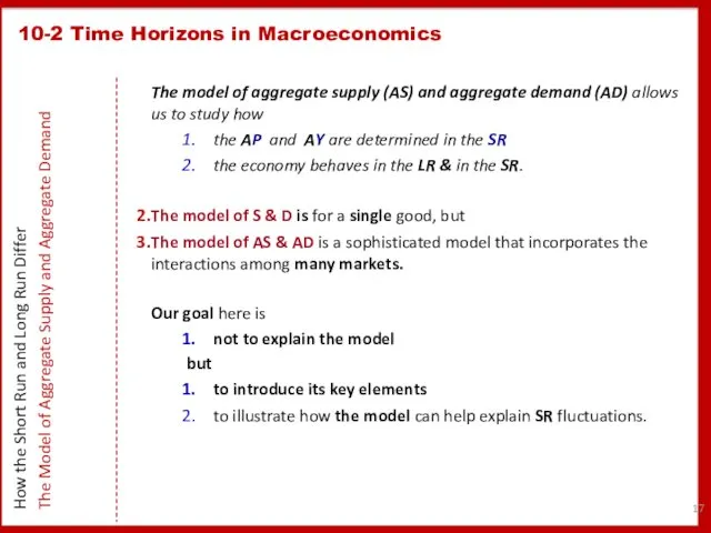
10-2 Time Horizons in Macroeconomics
How the Short Run and Long Run
10-2 Time Horizons in Macroeconomics
How the Short Run and Long Run
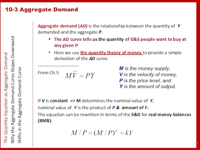
Aggregate demand (AD) is the relationship between the quantity of Y
Aggregate demand (AD) is the relationship between the quantity of Y
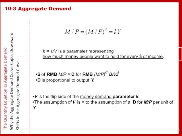
10-3 Aggregate Demand
The Quantity Equation as Aggregate Demand
Why the Aggregate Demand
10-3 Aggregate Demand
The Quantity Equation as Aggregate Demand
Why the Aggregate Demand
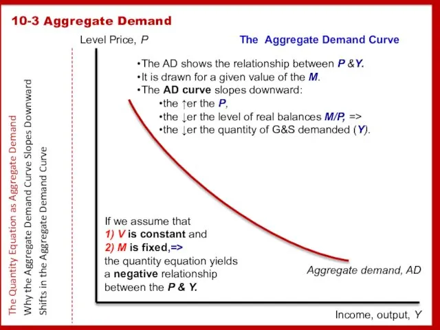
10-3 Aggregate Demand
The Quantity Equation as Aggregate Demand
Why the Aggregate Demand
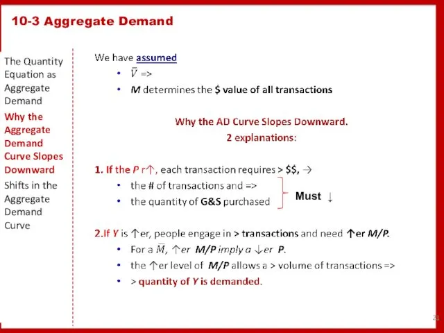
10-3 Aggregate Demand
The Quantity Equation as Aggregate Demand
Why the Aggregate Demand
10-3 Aggregate Demand
The Quantity Equation as Aggregate Demand
Why the Aggregate Demand
10-3 Aggregate Demand
The Quantity Equation as Aggregate Demand
Why the Aggregate Demand
10-3 Aggregate Demand
The Quantity Equation as Aggregate Demand
Why the Aggregate Demand
10-3 Aggregate Demand
The Quantity Equation as Aggregate Demand
Why the Aggregate Demand
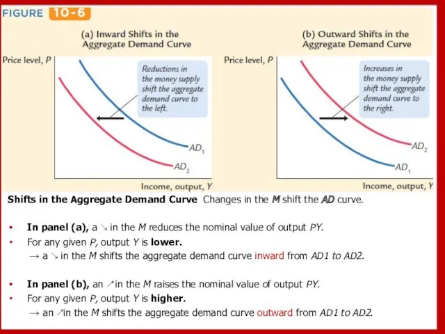
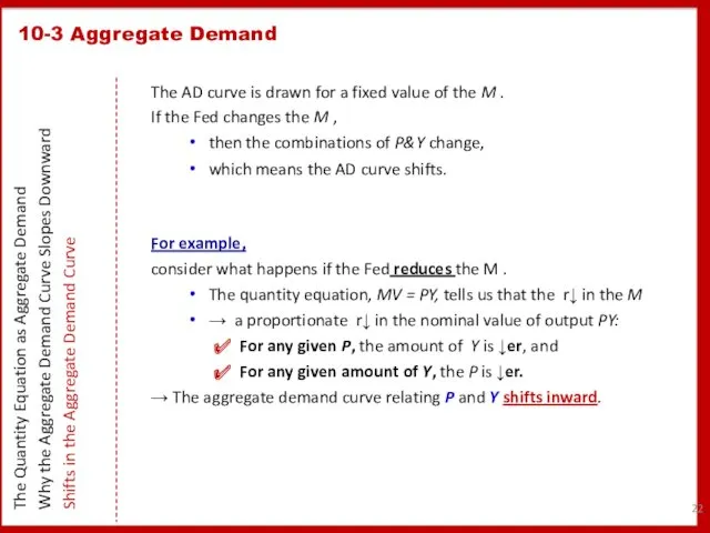
Shifts in the Aggregate Demand Curve Changes in the M shift
Shifts in the Aggregate Demand Curve Changes in the M shift
10-4 Aggregate Supply
The Long Run: The Vertical Aggregate Supply Curve
The Short
10-4 Aggregate Supply
The Long Run: The Vertical Aggregate Supply Curve
The Short
10-4 Aggregate Supply
The Long-Run Aggregate Supply Curve
In the lR, the
10-4 Aggregate Supply
The Long-Run Aggregate Supply Curve
In the lR, the
10-4 Aggregate Supply
Shifts in Aggregate Demand in the Long Run
A
10-4 Aggregate Supply
Shifts in Aggregate Demand in the Long Run
A
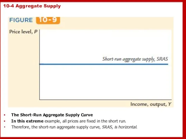
10-4 Aggregate Supply
The Short-Run Aggregate Supply Curve
In this extreme example,
10-4 Aggregate Supply
The Short-Run Aggregate Supply Curve
In this extreme example,
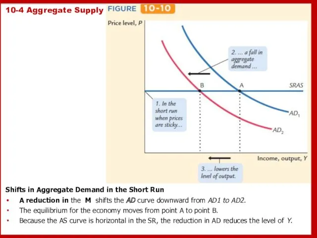
10-4 Aggregate Supply
Shifts in Aggregate Demand in the Short Run
A
10-4 Aggregate Supply
Shifts in Aggregate Demand in the Short Run
A
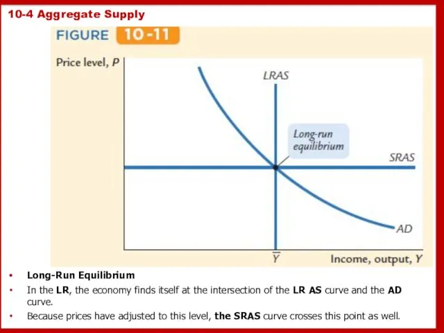
10-4 Aggregate Supply
Long-Run Equilibrium
In the LR, the economy finds itself
10-4 Aggregate Supply
Long-Run Equilibrium
In the LR, the economy finds itself
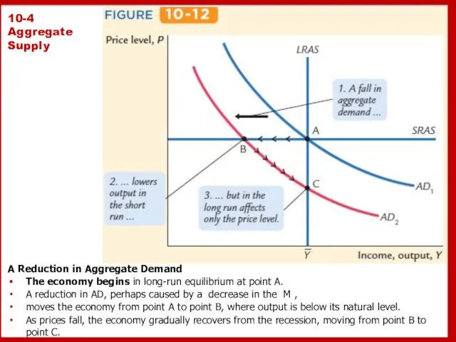
10-4 Aggregate Supply
A Reduction in Aggregate Demand
The economy begins in
10-4 Aggregate Supply
A Reduction in Aggregate Demand
The economy begins in
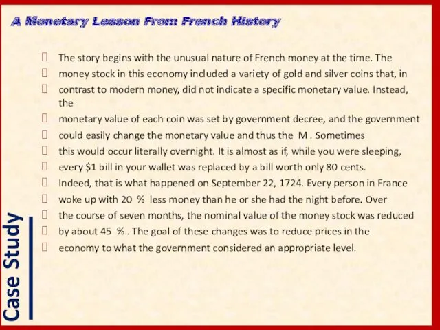
The story begins with the unusual nature of French money at
The story begins with the unusual nature of French money at
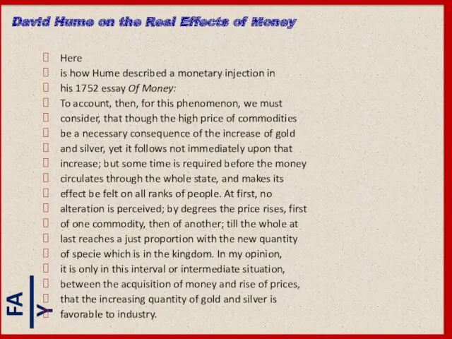
Here
is how Hume described a monetary injection in
his 1752 essay Of
Here
is how Hume described a monetary injection in
his 1752 essay Of
Fluctuations in the economy as a whole come from changes AS
10-5 Stabilization Policy
An Increase in Aggregate Demand
The economy begins
10-5 Stabilization Policy
An Increase in Aggregate Demand
The economy begins
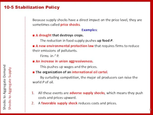
Because supply shocks have a direct impact on the price level,
Because supply shocks have a direct impact on the price level,
10-5 Stabilization Policy
An Adverse Supply Shock
An adverse supply shock
10-5 Stabilization Policy
An Adverse Supply Shock
An adverse supply shock
10-5 Stabilization Policy
Accommodating an Adverse Supply Shock
In response to
10-5 Stabilization Policy
Accommodating an Adverse Supply Shock
In response to
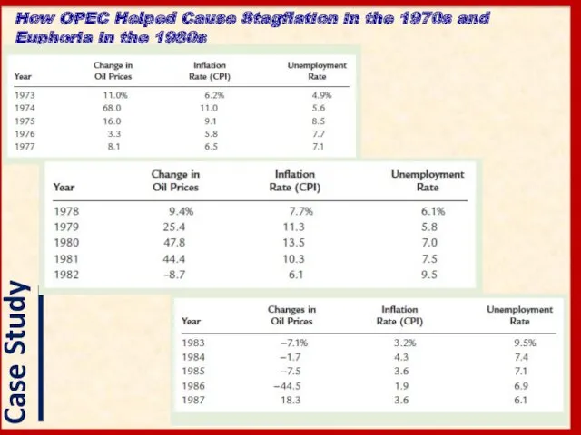
How OPEC Helped Cause Stagflation in the 1970s and Euphoria in
How OPEC Helped Cause Stagflation in the 1970s and Euphoria in
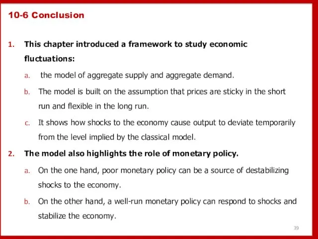
10-6 Conclusion
This chapter introduced a framework to study economic fluctuations:
the
10-6 Conclusion
This chapter introduced a framework to study economic fluctuations:
the
 Глобальные проблемы человечества
 Обзор рынка труда Ярославской области
 Статистические показатели, используемые в государственном регулировании
 Социальное государство
 Система национальных счетов. Основные макроэкономические показатели
 Фирма в условиях несовершенной конкуренции. (Лекция 5)
 Экономические циклы
 Презентация к уроку экономики Деньги: понятие, сущность, виды
 Экономическая сфера. Экономика как наука. Тема 3.1
 Спрос и предложение. Равновесная цена
 Німеччина - високорозвинена європейська країна
 Конкуренция, ее виды и особенности
 Основы рыночного хозяйства
 Организация и условия труда работников
 Система финансирования капитального ремонта
 Глобальные экономические проблемы
 Swiss Companies. The Swiss Limited Company‘s Example
 Показатели, которые будут прогнозироваться в разделе Потребительский рынок
 Конкуренция. Виды конкуренции
 Роль стандартов и технического регулирования в цементной отрасли
 Анализ объема производства и реализации товаров, услуг. (Тема 9)
 Мировой Экономический Кризис
 The costs of production. Income from factors of production
 Сельское хозяйство Австралии
 Decision time frames
 Поведение потребителя
 Нетарифное регулирование внешнеторговой деятельности в системе экономики таможенного дела
 Содержание предпринимательской деятельности