- Decision time frames

Содержание
- 2. Decision Time Frames The Short Run The short run is a time frame in which the
- 3. Decision Time Frames The Long Run The long run is a time frame in which the
- 4. Example With regard to economic decision making for firms, the short run is A) a definite
- 5. Example With regard to economic decision making for firms, the long run is a period in
- 6. Example Sandra has plans to go to an opera and already has a $100 non-refundable, non-exchangeable,
- 7. Short-Run Technology Constraint To increase output in the short run, a firm must increase the amount
- 8. Short-Run Technology Constraint Total product is the total output produced in a given period. The marginal
- 9. Total Product, Marginal Product, Average Product
- 10. Total Product It separates attainable output levels from unattainable output levels in the short run.
- 11. Figure 4: Total and Marginal Product 30 90 130 161 184 196 Total Product ΔQ from
- 12. Short-Run Technology Constraint Initially increasing marginal returns When the marginal product of a worker exceeds the
- 13. Short-Run Technology Constraint Increasing marginal returns arise from increased specialization and division of labor. Diminishing marginal
- 14. Example The following data show the total output for a firm when different amounts of labor
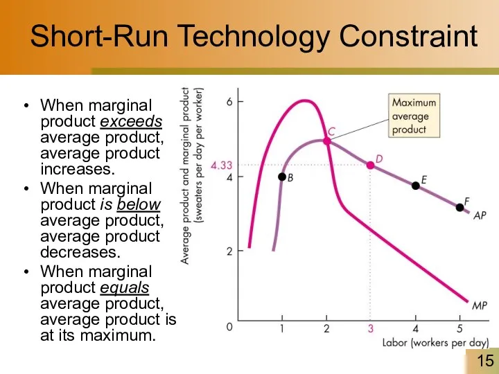
- 15. Short-Run Technology Constraint When marginal product exceeds average product, average product increases. When marginal product is
- 16. Example Consider a basket-producing firm with fixed capital. If the firm can produce 36 baskets per
- 17. Short-Run Cost To produce more output in the short run, the firm must employ more labor,
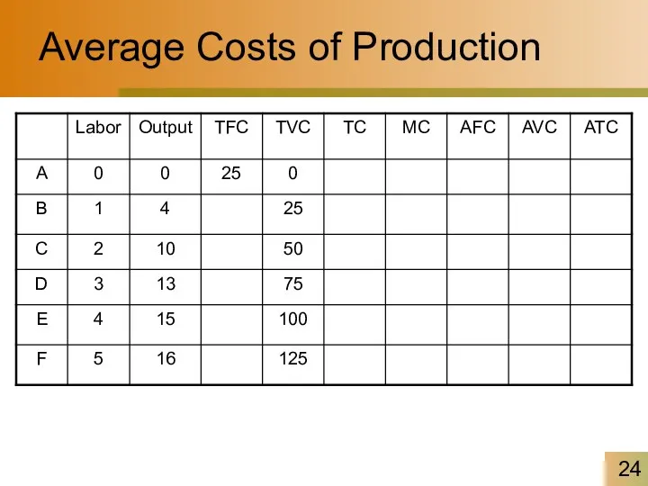
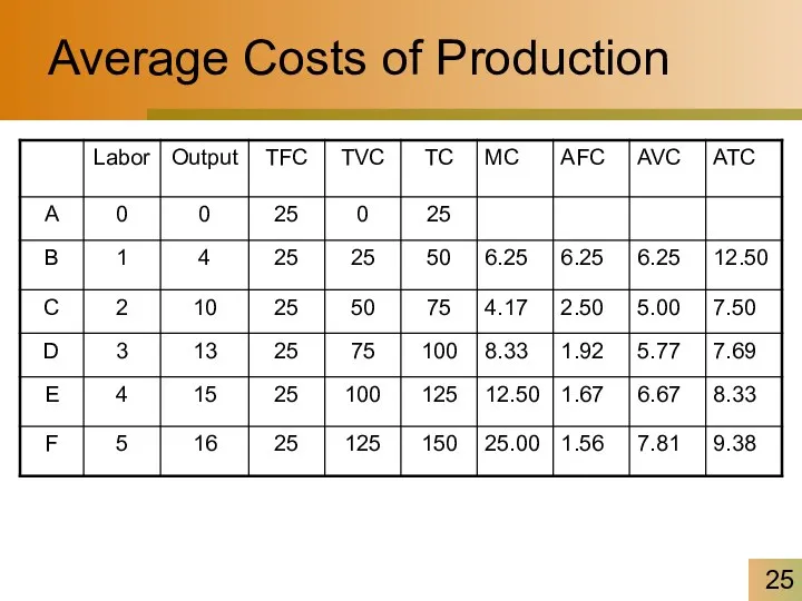
- 18. Short-Run Cost Total Cost A firm’s total cost (TC) is the cost of all resources used.
- 19. Total Costs of Production
- 20. Example Larry’s Performance Pizza is a small restaurant that sells low-carbohydrate pizzas in a health -
- 21. Total Costs of Production Total fixed cost is the same at each output level. Total variable
- 22. Short-Run Cost Marginal Cost Marginal cost (MC) is the increase in total cost that results from
- 23. Short-Run Cost Average Cost Average cost measures can be derived from each of the total cost
- 24. Average Costs of Production
- 25. Average Costs of Production
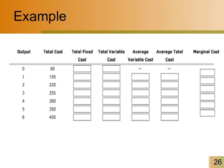
- 26. Example
- 27. Example The following data show the total output for a firm when specified amounts of labor
- 28. Average And Marginal Costs MC AVC ATC AFC
- 29. The Relationship Between Average And Marginal Costs At low levels of output, the MC curve lies
- 30. Example Suppose a firm producing digital cameras is operating such that marginal costs are higher than
- 31. Short-Run Cost Shifts in Cost Curves The position of a firm’s cost curves depend on two
- 32. Short-Run Cost Technological change influences both the productivity curves and the cost curves. An increase in
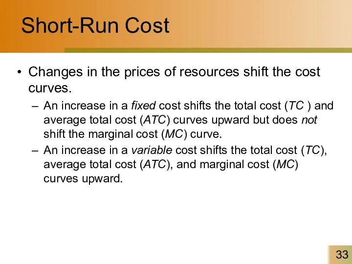
- 33. Short-Run Cost Changes in the prices of resources shift the cost curves. An increase in a
- 34. Example In the short run, when capital is a fixed factor, a rise in the cost
- 35. Production And Cost in the Long Run In the long run, costs behave differently Firm can
- 36. Production And Cost in the Long Run Long-run total cost The cost of producing each quantity
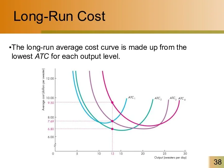
- 37. Long-Run Cost The average cost of producing a given output varies and depends on the firm’s
- 38. Long-Run Cost
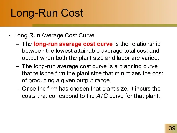
- 39. Long-Run Cost Long-Run Average Cost Curve The long-run average cost curve is the relationship between the
- 40. Long-Run Average Total Cost LRATC ATC1 Use 0 automated lines ATC3 ATC0 C B A ATC2
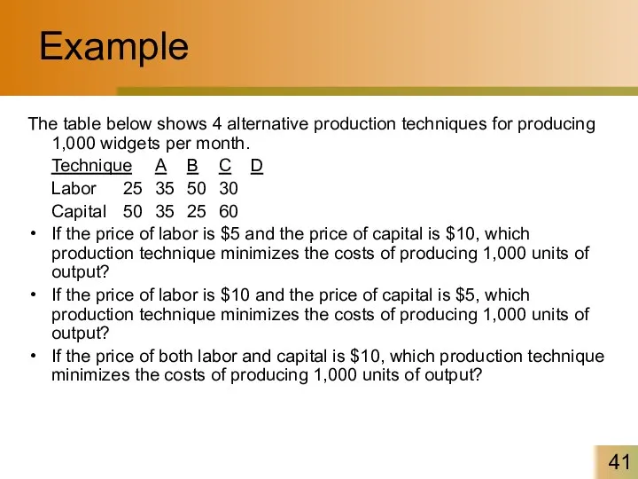
- 41. Example The table below shows 4 alternative production techniques for producing 1,000 widgets per month. Technique
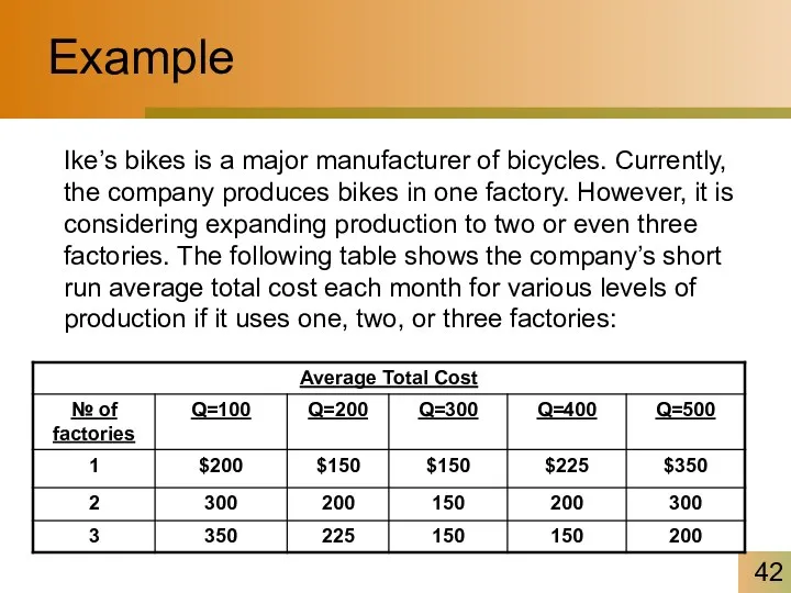
- 42. Example Ike’s bikes is a major manufacturer of bicycles. Currently, the company produces bikes in one
- 43. Example 1. Suppose Ike’s Bikes is currently producing 500 bikes per month in its (only) factory.
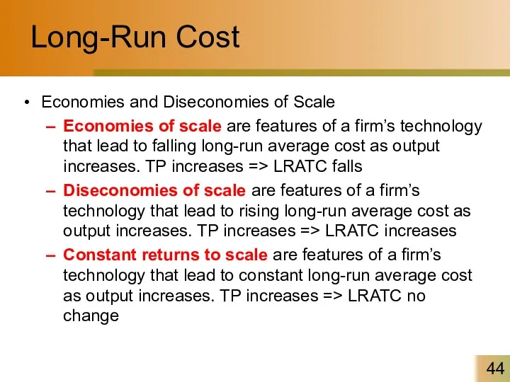
- 44. Long-Run Cost Economies and Diseconomies of Scale Economies of scale are features of a firm’s technology
- 45. The Shape Of LRATC Units of Output LRATC Economies of Scale Constant Returns to Scale Diseconomies
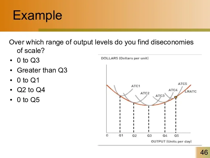
- 46. Example Over which range of output levels do you find diseconomies of scale? 0 to Q3
- 47. Long-Run Cost A firm experiences economies of scale up to some output level. Beyond that output
- 48. Returns to Scale In production, returns to scale refers to changes in output subsequent to a
- 49. Example Assume a firm is using 10 units of labor and 10 units of capital and
- 51. Скачать презентацию
Decision Time Frames
The Short Run
The short run is a time frame
Decision Time Frames
The Short Run
The short run is a time frame
Decision Time Frames
The Long Run
The long run is a time frame
Decision Time Frames
The Long Run
The long run is a time frame
Example
With regard to economic decision making for firms, the short run
Example
With regard to economic decision making for firms, the short run
Example
With regard to economic decision making for firms, the long run
Example
With regard to economic decision making for firms, the long run
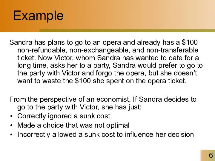
Example
Sandra has plans to go to an opera and already has
Example
Sandra has plans to go to an opera and already has
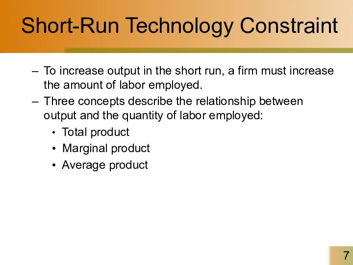
Short-Run Technology Constraint
To increase output in the short run, a firm
Short-Run Technology Constraint
To increase output in the short run, a firm
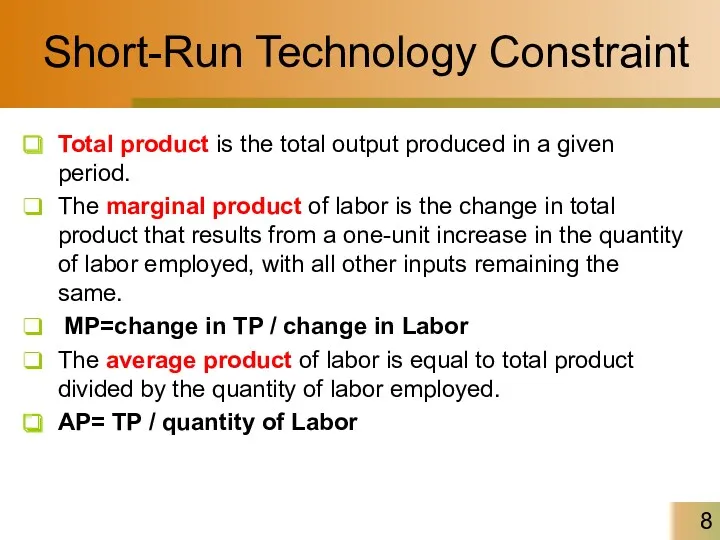
Short-Run Technology Constraint
Total product is the total output produced in a
Short-Run Technology Constraint
Total product is the total output produced in a
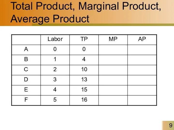
Total Product, Marginal Product, Average Product
Total Product, Marginal Product, Average Product
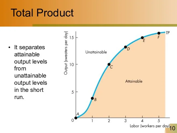
Total Product
It separates attainable output levels from unattainable output levels in
Total Product
It separates attainable output levels from unattainable output levels in
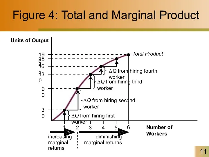
Figure 4: Total and Marginal Product
30
90
130
161
184
196
Total Product
ΔQ from hiring fourth worker
ΔQ
Figure 4: Total and Marginal Product
30
90
130
161
184
196
Total Product
ΔQ from hiring fourth worker
ΔQ
Short-Run Technology Constraint
Initially increasing marginal returns
When the marginal product of a
Short-Run Technology Constraint
Initially increasing marginal returns
When the marginal product of a

Short-Run Technology Constraint
Increasing marginal returns arise from increased specialization and division
Short-Run Technology Constraint
Increasing marginal returns arise from increased specialization and division
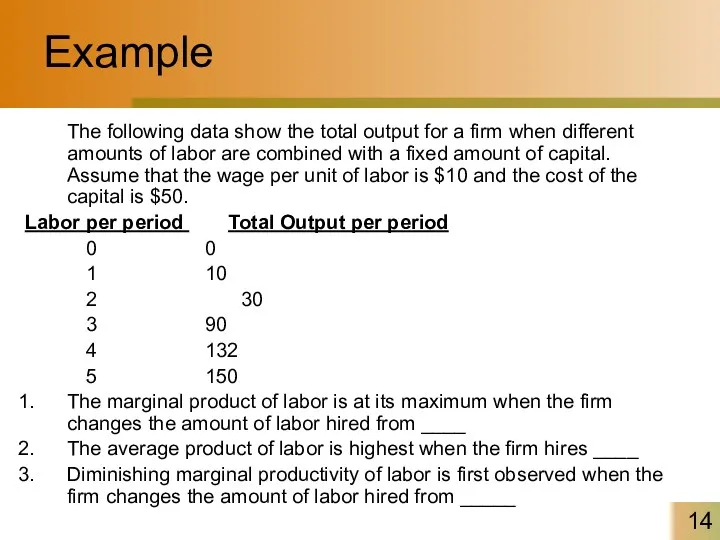
Example
The following data show the total output for a firm when
Example
The following data show the total output for a firm when
Short-Run Technology Constraint
When marginal product exceeds average product, average product increases.
When
Short-Run Technology Constraint
When marginal product exceeds average product, average product increases.
When
Example
Consider a basket-producing firm with fixed capital. If the firm can
Example
Consider a basket-producing firm with fixed capital. If the firm can
Short-Run Cost
To produce more output in the short run, the firm
Short-Run Cost
To produce more output in the short run, the firm

Short-Run Cost
Total Cost
A firm’s total cost (TC) is the cost of
Short-Run Cost
Total Cost
A firm’s total cost (TC) is the cost of
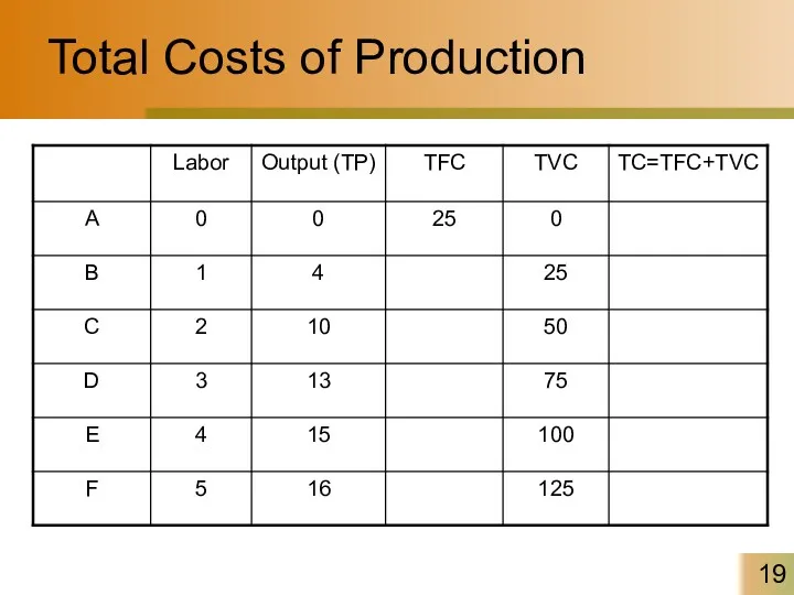
Total Costs of Production
Total Costs of Production
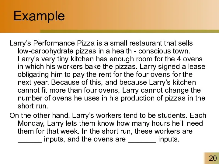
Example
Larry’s Performance Pizza is a small restaurant that sells low-carbohydrate pizzas
Example
Larry’s Performance Pizza is a small restaurant that sells low-carbohydrate pizzas
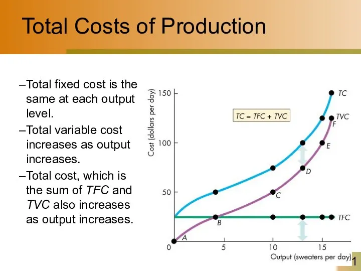
Total Costs of Production
Total fixed cost is the same at each
Total Costs of Production
Total fixed cost is the same at each
Short-Run Cost
Marginal Cost
Marginal cost (MC) is the increase in total cost
Short-Run Cost
Marginal Cost
Marginal cost (MC) is the increase in total cost
Short-Run Cost
Average Cost
Average cost measures can be derived from each of
Short-Run Cost
Average Cost
Average cost measures can be derived from each of
Average Costs of Production
Average Costs of Production
Average Costs of Production
Average Costs of Production
Example
Example
Example
The following data show the total output for a firm when
Example
The following data show the total output for a firm when
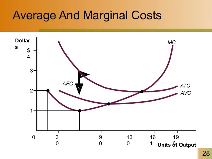
Average And Marginal Costs
MC
AVC
ATC
AFC
Average And Marginal Costs
MC
AVC
ATC
AFC
The Relationship Between Average And Marginal Costs
At low levels of output,
The Relationship Between Average And Marginal Costs
At low levels of output,
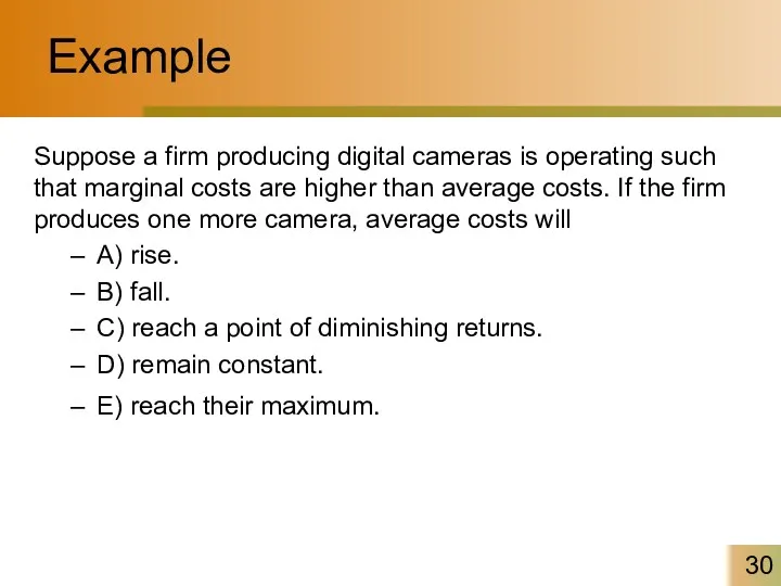
Example
Suppose a firm producing digital cameras is operating such that marginal
Example
Suppose a firm producing digital cameras is operating such that marginal
Short-Run Cost
Shifts in Cost Curves
The position of a firm’s cost curves
Short-Run Cost
Shifts in Cost Curves
The position of a firm’s cost curves

Short-Run Cost
Technological change influences both the productivity curves and the cost
Short-Run Cost
Technological change influences both the productivity curves and the cost
Short-Run Cost
Changes in the prices of resources shift the cost curves.
An
Short-Run Cost
Changes in the prices of resources shift the cost curves.
An
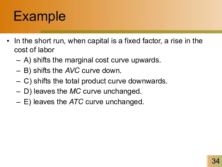
Example
In the short run, when capital is a fixed factor, a
Example
In the short run, when capital is a fixed factor, a
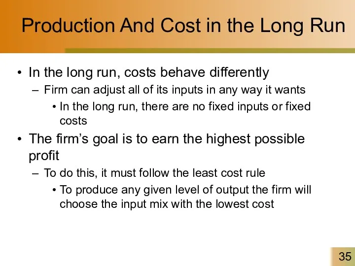
Production And Cost in the Long Run
In the long run, costs
Production And Cost in the Long Run
In the long run, costs
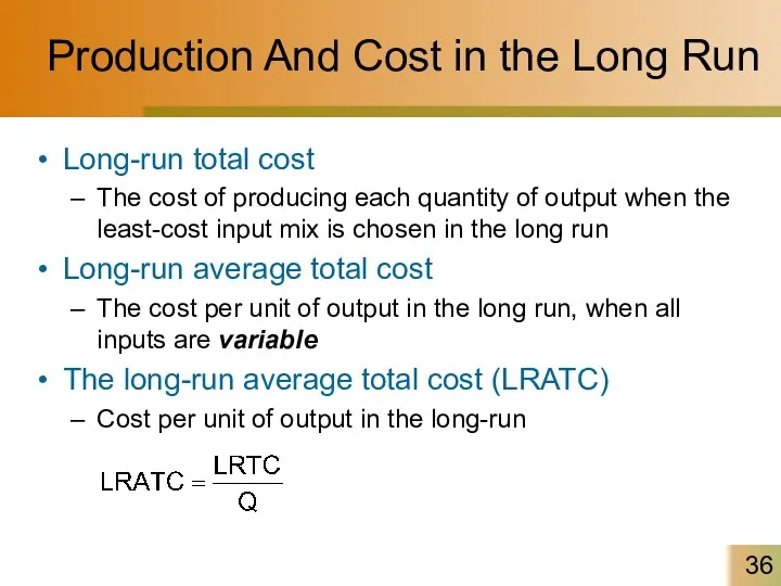
Production And Cost in the Long Run
Long-run total cost
The cost of
Production And Cost in the Long Run
Long-run total cost
The cost of
Long-Run Cost
The average cost of producing a given output varies and
Long-Run Cost
The average cost of producing a given output varies and
Long-Run Cost
Long-Run Cost
Long-Run Cost
Long-Run Average Cost Curve
The long-run average cost curve is the
Long-Run Cost
Long-Run Average Cost Curve
The long-run average cost curve is the
Long-Run Average Total Cost
LRATC
ATC1
Use 0 automated lines
ATC3
ATC0
C
B
A
ATC2
D
E
175
Use 1 automated lines
Use 2
Long-Run Average Total Cost
LRATC
ATC1
Use 0 automated lines
ATC3
ATC0
C
B
A
ATC2
D
E
175
Use 1 automated lines
Use 2
Example
The table below shows 4 alternative production techniques for producing 1,000
Example
The table below shows 4 alternative production techniques for producing 1,000
Example
Ike’s bikes is a major manufacturer of bicycles. Currently, the company
Example
Ike’s bikes is a major manufacturer of bicycles. Currently, the company

Example
1. Suppose Ike’s Bikes is currently producing 500 bikes per month in
Example
1. Suppose Ike’s Bikes is currently producing 500 bikes per month in
Long-Run Cost
Economies and Diseconomies of Scale
Economies of scale are features of
Long-Run Cost
Economies and Diseconomies of Scale
Economies of scale are features of
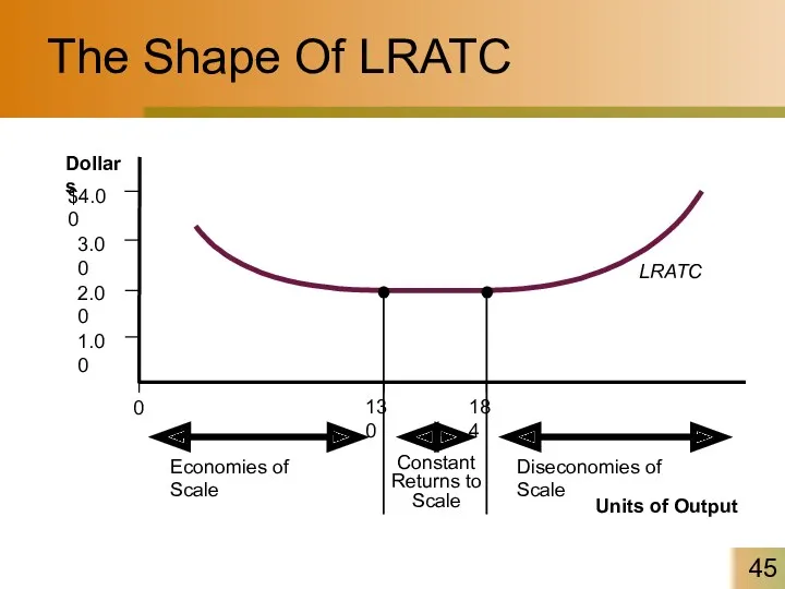
The Shape Of LRATC
Units of Output
LRATC
Economies of Scale
Constant Returns to Scale
Diseconomies
The Shape Of LRATC
Units of Output
LRATC
Economies of Scale
Constant Returns to Scale
Diseconomies
Example
Over which range of output levels do you find diseconomies of
Example
Over which range of output levels do you find diseconomies of
Long-Run Cost
A firm experiences economies of scale up to some output
Long-Run Cost
A firm experiences economies of scale up to some output
Returns to Scale
In production, returns to scale refers to changes in
Returns to Scale
In production, returns to scale refers to changes in
Example
Assume a firm is using 10 units of labor and 10
Example
Assume a firm is using 10 units of labor and 10
 Impact of globalization on local culture
 Спрос и предложение на рынке труда
 Развитие экспортного потенциала культурных и креативных индустрий в Европейском союзе
 Индикаторы устойчивого развития-2
 Человек в мире экономических отношений
 Международные валютные отношения и валютный рынок. (Темы 1-2) Валюта как ключевая категория международных валютных отношений
 Теории эластичности спроса и предложения
 Макроэкономическая нестабильность. Безработица и занятость (макроэкономические показатели)
 Організація та технологія надання пасажирських послуг
 Өндіріс факторларының нарығы
 Альтерглобалізм та його форми
 Экономика и государство
 Кейнсианство. Джон Мейнард Кейнс
 Производственная программа и производственные мощности. Экономика организации. (Лекция 7)
 Цели, организация и методы антимонопольного регулирования
 Анализ возможностей выхода ПАО Газпром на Азиатско-тихоокеанские рынки
 Спрос. Закон спроса. Эластичность спроса
 Підприємницька ідея: механізм генерування та впровадження
 Место Китая в мировом хозяйстве
 Экономика организации. Трудовые ресурсы организации. Основы организации труда и его оплаты
 Анализ рынка СЭД в РФ
 Әлеуметтік – экономикалық дамудағы дағдарыс түсінігі және оның пайда болу себептері
 Рыночная экономика. Тема 14. Обществознание. 8 класс
 Фінансові ресурси торговельного підприємства. (Лекція 11)
 Тема 10. Экономическая роль государства
 Рынки факторов производства
 Риск в экономике
 История создания ГАТТ/ВТО. Организационная структура ВТО