- Demand 11.2a

Содержание
- 2. Learning Objectives By the end of the lesson the learners will be able to : Define
- 3. Demand Willingness to Buy Ability to Pay
- 4. Demand Schedule 01/11/2016 Sonali Sinha Roy
- 5. Downward slope of Demand Curve 01/11/2016 Sonali Sinha Roy Law of Demand: The negative relationship between
- 6. Reason for Downward Sloping Demand Curve 01/11/2016 Sonali Sinha Roy The negative slope of the demand
- 7. Movement along the Demand Curve 01/11/2016 Sonali Sinha Roy Movement along the Demand curve is due
- 8. Shift in Demand 01/11/2016 Sonali Sinha Roy PINTE: P = Price of the related goods I
- 9. Identify from the following: Normal & Inferior Goods ; Complementary & Substitute Goods 01/11/2016 Sonali Sinha
- 10. Shifts in Demand Curve 01/11/2016 Sonali Sinha Roy
- 11. 01/11/2016 Sonali Sinha Roy
- 12. Recap of Today’s Lesson 01/11/2016 Sonali Sinha Roy
- 13. Reflection 01/11/2016 Sonali Sinha Roy
- 14. Demand 11.2a Lesson 2 NIS 01/11/2016 Sonali Sinha Roy
- 15. Learning Objectives By the end of the lesson the learners will be able to : Define
- 16. Demand Function 01/11/2016 Sonali Sinha Roy Indirect relationship between Price and Quantity Demanded QD P Equation:
- 17. Example 01/11/2016 Sonali Sinha Roy Demand: Q = 100 -2P Inverse Demand: P = 50 –
- 18. In-class activity 01/11/2016 Sonali Sinha Roy Use the linear demand function for cappuccinos, Qd = 500
- 19. Recap of Today’s Lesson 01/11/2016 Sonali Sinha Roy
- 21. Скачать презентацию
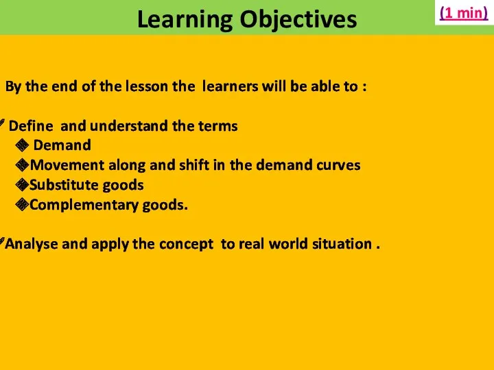
Learning Objectives
By the end of the lesson the learners will
Learning Objectives
By the end of the lesson the learners will

Demand
Willingness to Buy
Ability to Pay
Demand
Willingness to Buy
Ability to Pay
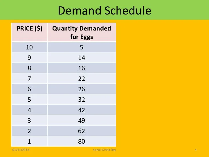
Demand Schedule
01/11/2016
Sonali Sinha Roy
Demand Schedule
01/11/2016
Sonali Sinha Roy
Downward slope of Demand Curve
01/11/2016
Sonali Sinha Roy
Law of Demand:
The negative
Downward slope of Demand Curve
01/11/2016
Sonali Sinha Roy
Law of Demand:
The negative
Reason for Downward Sloping Demand Curve
01/11/2016
Sonali Sinha Roy
The negative slope of
Reason for Downward Sloping Demand Curve
01/11/2016
Sonali Sinha Roy
The negative slope of
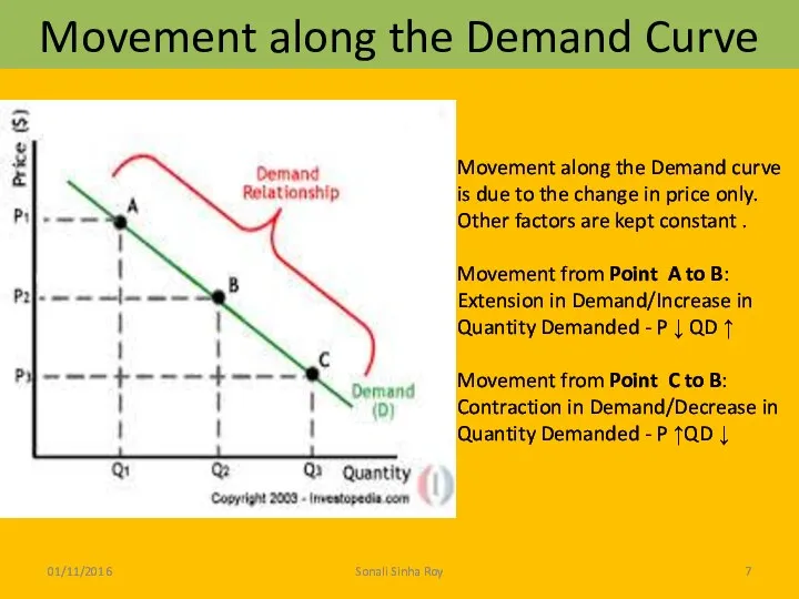
Movement along the Demand Curve
01/11/2016
Sonali Sinha Roy
Movement along the Demand curve
Movement along the Demand Curve
01/11/2016
Sonali Sinha Roy
Movement along the Demand curve

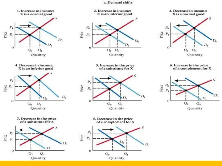
Shift in Demand
01/11/2016
Sonali Sinha Roy
PINTE:
P = Price of the related
Shift in Demand
01/11/2016
Sonali Sinha Roy
PINTE:
P = Price of the related
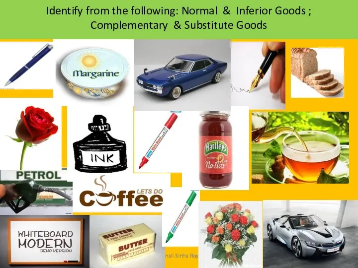
Identify from the following: Normal & Inferior Goods ;
Complementary &
Identify from the following: Normal & Inferior Goods ; Complementary &
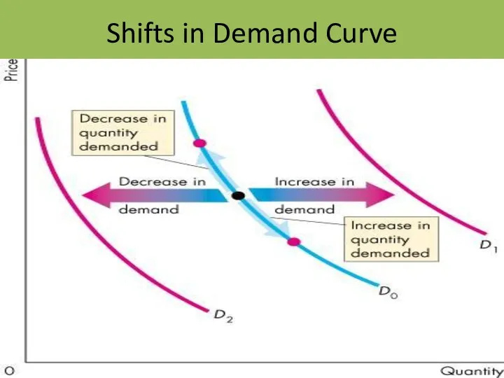
Shifts in Demand Curve
01/11/2016
Sonali Sinha Roy
Shifts in Demand Curve
01/11/2016
Sonali Sinha Roy
01/11/2016
Sonali Sinha Roy
01/11/2016
Sonali Sinha Roy

Recap of Today’s Lesson
01/11/2016
Sonali Sinha Roy
Recap of Today’s Lesson
01/11/2016
Sonali Sinha Roy

Reflection
01/11/2016
Sonali Sinha Roy
Reflection
01/11/2016
Sonali Sinha Roy
Demand
11.2a
Lesson 2
NIS
01/11/2016
Sonali Sinha Roy
Demand
11.2a
Lesson 2
NIS
01/11/2016
Sonali Sinha Roy

Learning Objectives
By the end of the lesson the learners will
Learning Objectives
By the end of the lesson the learners will
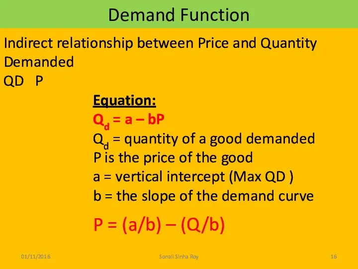
Demand Function
01/11/2016
Sonali Sinha Roy
Indirect relationship between Price and Quantity Demanded
Demand Function
01/11/2016
Sonali Sinha Roy
Indirect relationship between Price and Quantity Demanded
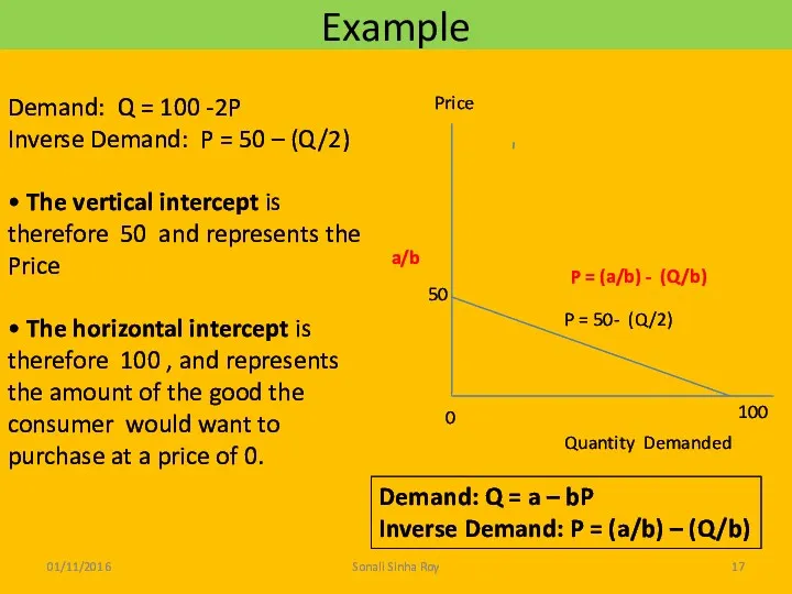
Example
01/11/2016
Sonali Sinha Roy
Demand: Q = 100 -2P
Inverse Demand: P = 50
Example
01/11/2016
Sonali Sinha Roy
Demand: Q = 100 -2P
Inverse Demand: P = 50

In-class activity
01/11/2016
Sonali Sinha Roy
Use the linear demand function for cappuccinos, Qd =
In-class activity
01/11/2016
Sonali Sinha Roy
Use the linear demand function for cappuccinos, Qd =
Recap of Today’s Lesson
01/11/2016
Sonali Sinha Roy
Recap of Today’s Lesson
01/11/2016
Sonali Sinha Roy
 Счета доходов
 Неравенство в Европе в 1990-2016 годах
 Рыночная система спроса и предложения
 Презентация по теме Зачем нужна биржа
 Экспо-2017 халықаралық көрмесін өткізетін
 Выступление генерального директора Россети Центр
 Unternehmertum in Belarus
 Структурные особенности экономики России
 Международная торговля. Государственная политика в области международной торговли
 Основы рыночной экономики. Рынок: его сущность
 Экономика
 Организационно-правовые формы предприятий. (Лекция 2)
 Рынок и рыночный механизм. Спрос и предложение. Издержки
 Норвегия. Уровень жизни в подробностях
 Отчёт о результатах деятельности главы и администрации городского округа Новокуйбышевск
 Глобальные проблемы человечества: энергетическая проблема
 Курсовая работа по дисциплине “Экономика организации”
 Сегмент упаковки в экономике замкнутого цикла
 Спрос, предложение, цена
 Экономика России в начале XXI века
 Информатизация отрасли ЖКХ. (Тема 13)
 Исследования эффективности солнечной энергетики в Крыму
 Туристическое агентство ТУР-ФОРТИНС
 Системный анализ в экономике. Технология прикладного системного анализа (ПСА)
 Основные фонды предприятия
 Стратегия развития железнодорожного транспорта в РФ до 2030 года
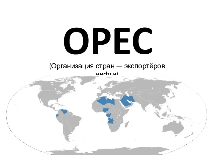 Организация стран — экспортёров нефти (OPEC)
 Рынок образовательных услуг