- Supply 11.2a

Содержание
- 2. Learning Objectives By the end of the lesson the learners will be able to : Define
- 3. Willingness to sell product at various given prices at a given point of time sUPPLY 01/11/2016
- 4. Supply Curve 01/11/2016 Sonali Sinha Roy
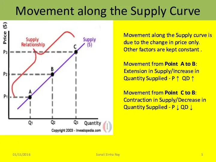
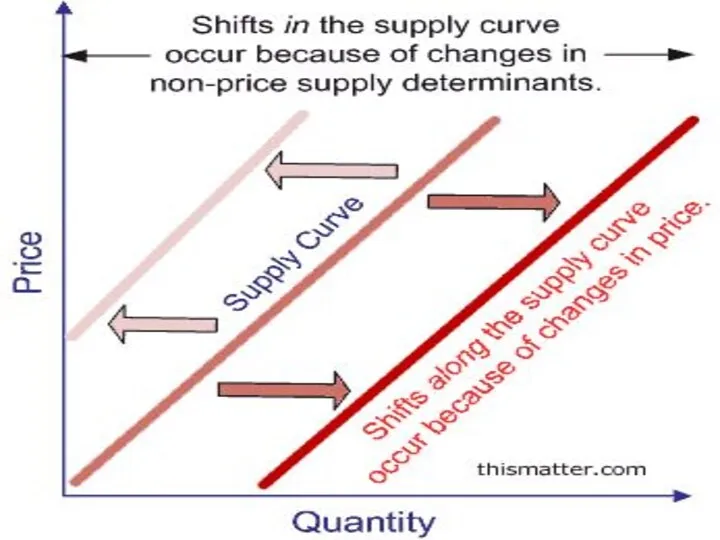
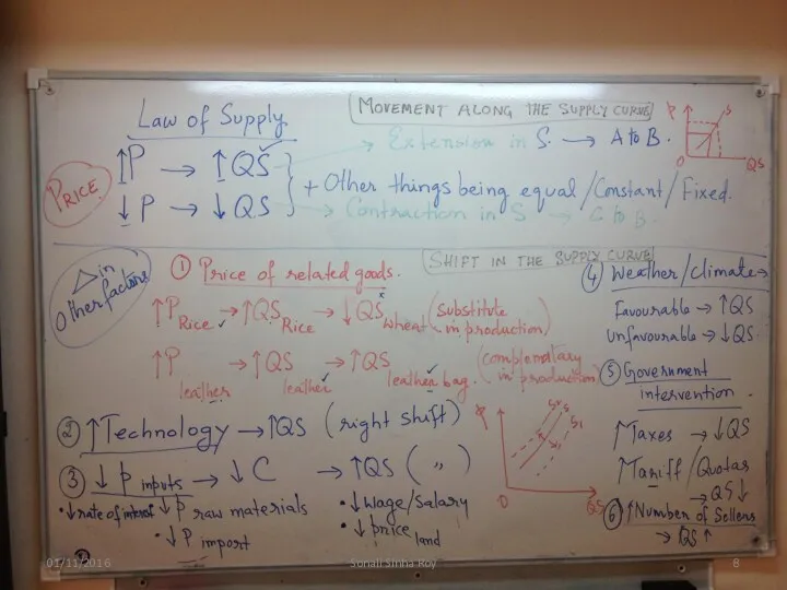
- 5. 01/11/2016 Sonali Sinha Roy Movement along the Supply Curve Movement along the Supply curve is due
- 6. 01/11/2016 Sonali Sinha Roy
- 7. Shifts in supply curve 01/11/2016 Sonali Sinha Roy SPENT S = Supplier prices (FOP) P =
- 8. 01/11/2016 Sonali Sinha Roy
- 9. 01/11/2016 Sonali Sinha Roy
- 10. Supply curve shifts to the right 01/11/2016 Sonali Sinha Roy Why might the supply curve shift
- 11. Supply curve shifts to the left 01/11/2016 Sonali Sinha Roy Why might the supply curve shift
- 12. Example: Case Study 01/11/2016 Sonali Sinha Roy
- 13. Recap of Today’s Lesson 01/11/2016 Sonali Sinha Roy
- 14. Reflection 01/11/2016 Sonali Sinha Roy
- 15. Supply 11.2a Lesson 4 NIS 01/11/2016 Sonali Sinha Roy
- 16. Learning Objectives By the end of the lesson the learners will be able to : Define
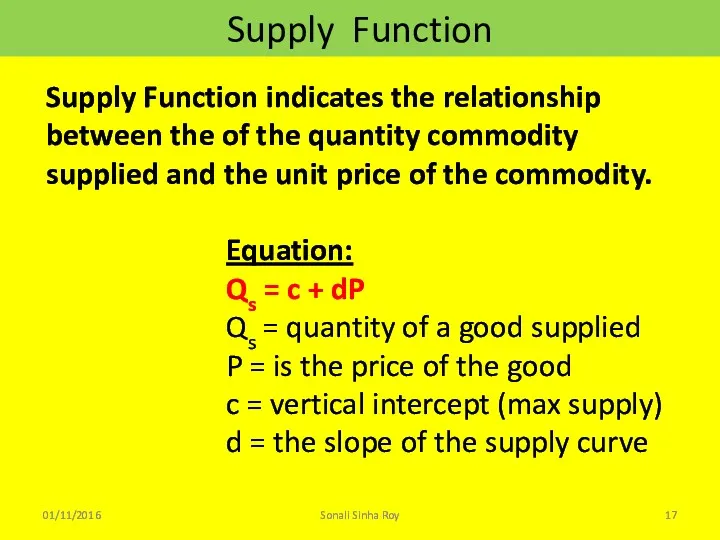
- 17. Supply Function 01/11/2016 Sonali Sinha Roy Supply Function indicates the relationship between the of the quantity
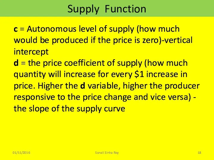
- 18. Supply Function 01/11/2016 Sonali Sinha Roy c = Autonomous level of supply (how much would be
- 19. 01/11/2016 Sonali Sinha Roy Example
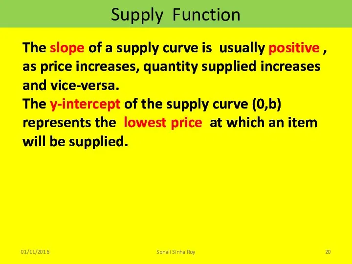
- 20. Supply Function 01/11/2016 Sonali Sinha Roy The slope of a supply curve is usually positive ,
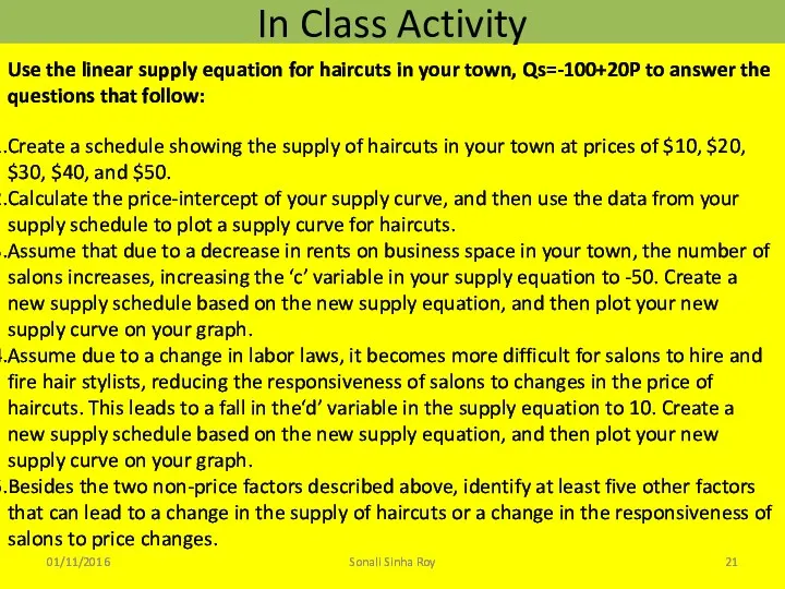
- 21. In Class Activity 01/11/2016 Sonali Sinha Roy Use the linear supply equation for haircuts in your
- 22. Recap of Today’s Lesson 01/11/2016 Sonali Sinha Roy
- 24. Скачать презентацию
Learning Objectives
By the end of the lesson the learners will
Learning Objectives
By the end of the lesson the learners will
Willingness to sell product at various given prices at a given
Willingness to sell product at various given prices at a given
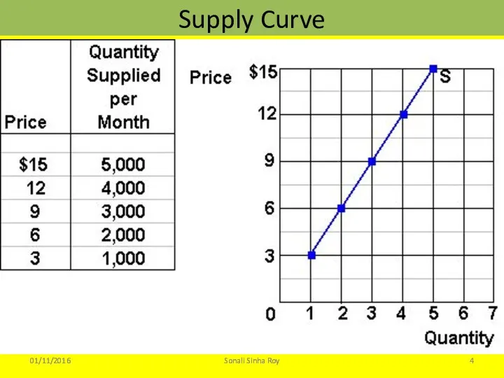
Supply Curve
01/11/2016
Sonali Sinha Roy
Supply Curve
01/11/2016
Sonali Sinha Roy
01/11/2016
Sonali Sinha Roy
Movement along the Supply Curve
Movement along the Supply curve
01/11/2016
Sonali Sinha Roy
Movement along the Supply Curve
Movement along the Supply curve
01/11/2016
Sonali Sinha Roy
01/11/2016
Sonali Sinha Roy
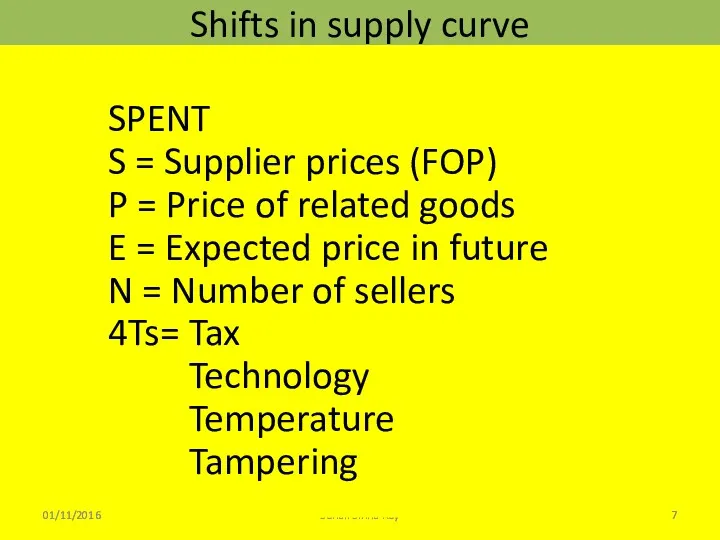
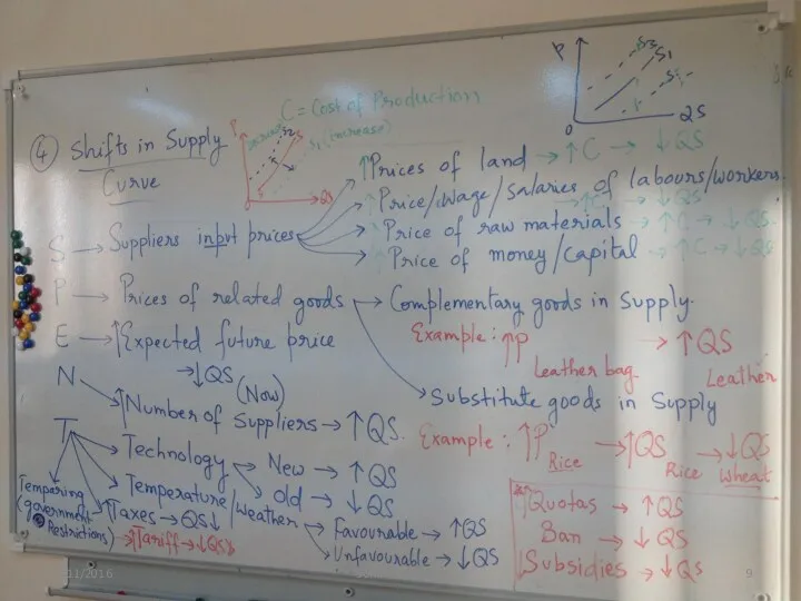
Shifts in supply curve
01/11/2016
Sonali Sinha Roy
SPENT
S = Supplier prices (FOP)
P =
Shifts in supply curve
01/11/2016
Sonali Sinha Roy
SPENT
S = Supplier prices (FOP)
P =
01/11/2016
Sonali Sinha Roy
01/11/2016
Sonali Sinha Roy
01/11/2016
Sonali Sinha Roy
01/11/2016
Sonali Sinha Roy
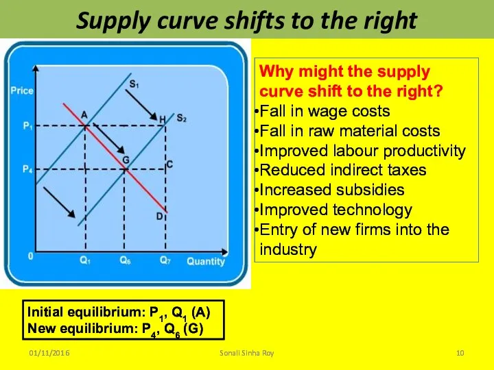
Supply curve shifts to the right
01/11/2016
Sonali Sinha Roy
Why might the supply
Supply curve shifts to the right
01/11/2016
Sonali Sinha Roy
Why might the supply
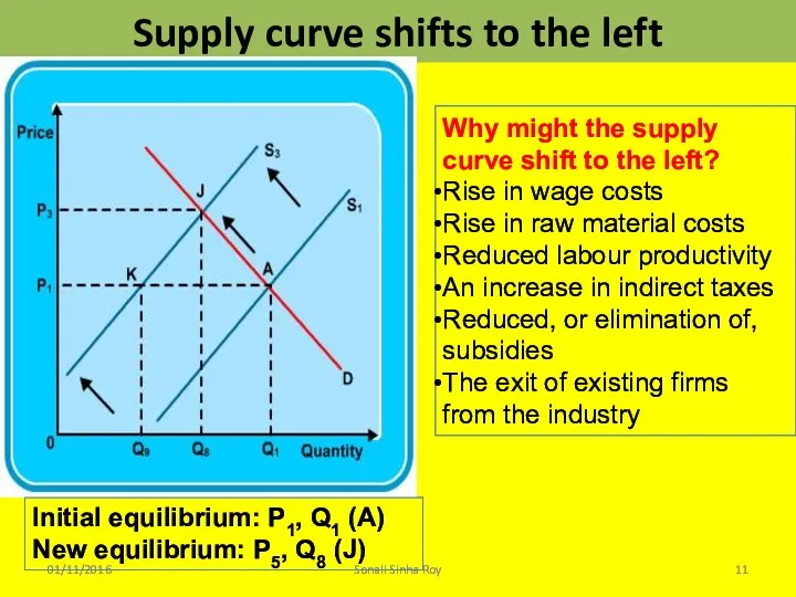
Supply curve shifts to the left
01/11/2016
Sonali Sinha Roy
Why might the supply
Supply curve shifts to the left
01/11/2016
Sonali Sinha Roy
Why might the supply
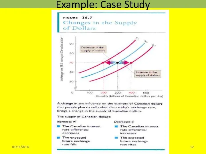
Example: Case Study
01/11/2016
Sonali Sinha Roy
Example: Case Study
01/11/2016
Sonali Sinha Roy
Recap of Today’s Lesson
01/11/2016
Sonali Sinha Roy
Recap of Today’s Lesson
01/11/2016
Sonali Sinha Roy

Reflection
01/11/2016
Sonali Sinha Roy
Reflection
01/11/2016
Sonali Sinha Roy
Supply
11.2a
Lesson 4
NIS
01/11/2016
Sonali Sinha Roy
Supply
11.2a
Lesson 4
NIS
01/11/2016
Sonali Sinha Roy
Learning Objectives
By the end of the lesson the learners will
Learning Objectives
By the end of the lesson the learners will
Supply Function
01/11/2016
Sonali Sinha Roy
Supply Function indicates the relationship between the
Supply Function
01/11/2016
Sonali Sinha Roy
Supply Function indicates the relationship between the
Supply Function
01/11/2016
Sonali Sinha Roy
c = Autonomous level of supply (how
Supply Function
01/11/2016
Sonali Sinha Roy
c = Autonomous level of supply (how

01/11/2016
Sonali Sinha Roy
Example
01/11/2016
Sonali Sinha Roy
Example
Supply Function
01/11/2016
Sonali Sinha Roy
The slope of a supply curve is
Supply Function
01/11/2016
Sonali Sinha Roy
The slope of a supply curve is
In Class Activity
01/11/2016
Sonali Sinha Roy
Use the linear supply equation for haircuts
In Class Activity
01/11/2016
Sonali Sinha Roy
Use the linear supply equation for haircuts

Recap of Today’s Lesson
01/11/2016
Sonali Sinha Roy
Recap of Today’s Lesson
01/11/2016
Sonali Sinha Roy
 Стратегия развития культуры Мариинского муниципального района на 2018-2035 гг
 Презентация к теме Реклама История рекламы от древности до наших дней
 Ұлттық экономика: мазмұны, құрылымы және нәтижесін өлшеу
 Национальное хозяйство (экономика) России. 9 класс
 Экономика и технологические уклады. Сущность экономической деятельности
 Изменение роли инновационной деятельности на разных этапах экономического развития
 Соціальні цілі економіки
 Макроэкономика. Национальный продукт и его измерение
 Деловой климат в странах СНГ. Методологический аспект оценки потенциала сотрудничества
 Основные фонды, основные средства, основной капитал
 Инфляция и антиинфляционная политика
 Инфляция, проблемы безработицы
 Рынок и его функции
 Экономика России
 История экономических учений
 Институциональная теория государства
 Экономическая организация общества
 О социально-экономическом развитии Беломорского муниципального района по итогам 2021 года и задачах на 2022 год
 Экономика Японии
 Employment and Unemployment. Inflation
 Контроллинг как интегративная функция и инструментальная среда управления
 Ауыл шаруашылығының жалпы өнім көлемі, млрд. теңге
 Формування засад ринкового господарства в Україні (90-ті роки ХХ ст. та початок XXI cт.)
 Выталкивающая и вытягивающая системы планирования
 Теории регионального экономического развития
 Сегментация рынка
 Теория транспортных систем. Переходные процессы от командно-административной системы к рыночной экономике
 Государственная программа Развитие здравоохранения