- Training course in revenue forecasting

Содержание
- 2. Revenue Forecasting - Day Three - Overview Taxation and the Economy Tax Elasticity and Tax Buoyancy
- 3. Revenue Forecasting – Session 1 Stylized flow of funds within the macro-economy Macro-economic identities Tax revenue
- 4. The economic activity of any country can be represented by the flow of funds within that
- 5. Stylized flows of funds within the macro-economy X = Exports Taxes on G Government Consumption Purchases
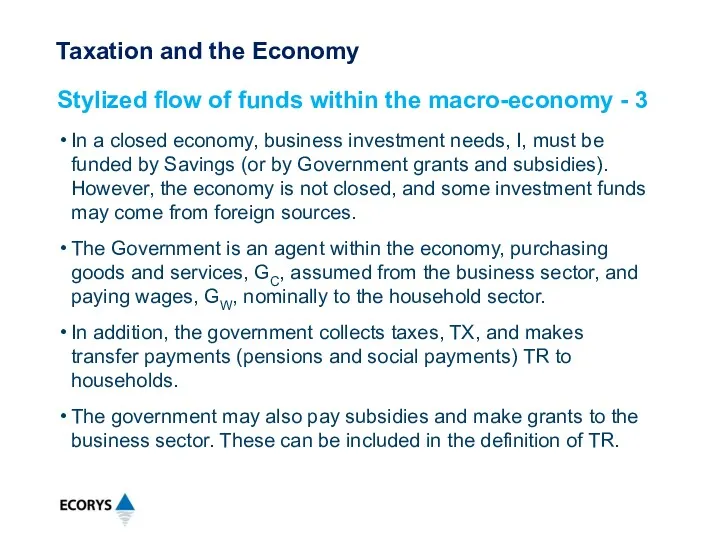
- 6. In a closed economy, business investment needs, I, must be funded by Savings (or by Government
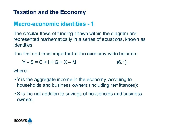
- 7. The circular flows of funding shown within the diagram are represented mathematically in a series of
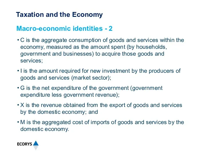
- 8. C is the aggregate consumption of goods and services within the economy, measured as the amount
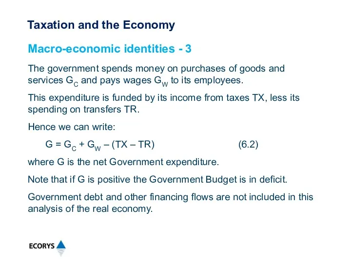
- 9. The government spends money on purchases of goods and services GC and pays wages GW to
- 10. The main flows of funds that have the potential to produce tax revenues are: gross income,
- 11. Major streams not taxed are: remittances (which form part of household income, and feed into household
- 12. Consumption and other indirect taxes Value Added Tax Private final consumption (household and small businesses) Excises
- 13. Income and other direct taxes Corporate income tax Operating surplus of (profits tax) incorporated entities Personal
- 14. Revenue Forecasting – Session 2 Definitions of tax buoyancy and tax elasticity Differences between tax buoyancy
- 15. Tax Buoyancy Tax buoyancy measures the total response of tax revenues to changes in national income
- 16. Tax Elasticity Tax elasticity measures the pure response of tax revenues to changes in the national
- 17. Tax buoyancy is the most appropriate measure when assessing the impact of tax policy and tax
- 18. Tax buoyancy can be expressed as follows: EbY = ( Δ Tb / Δ Y )
- 19. Tax elasticities are simpler to calculate than tax buoyancies, but they require the tax revenue series
- 20. An alternative way of writing this expression is: EY = ( %ΔT / %ΔY ) where:
- 21. Each of the measures, Buoyancy and Elasticity, may have values less than unity, equal to unity,
- 22. When tax policy changes have increased effective tax rates, such as an increase in the rate
- 23. Firstly, in terms of elasticity of taxes relative to GDP or its relevant main components, the
- 24. In periods of higher investment, the capital allowances reduce taxable income growth relative to the growth
- 25. Value Added Taxes (VAT) tend to have E ~ 1.0, relative to GDP as a whole
- 26. Excise Taxes (and Customs Duties) fall into two categories, with different elasticity expectations. For excise taxes
- 27. The second category includes the following For excisable goods subject to ad valorem excises (a percentage
- 28. For all taxes, excises and duties, individually and collectively, the buoyancy will be higher than the
- 29. Revenue Forecasting – Session 3 General approach to forecasting revenues using forecasts of macroeconomic variables Example
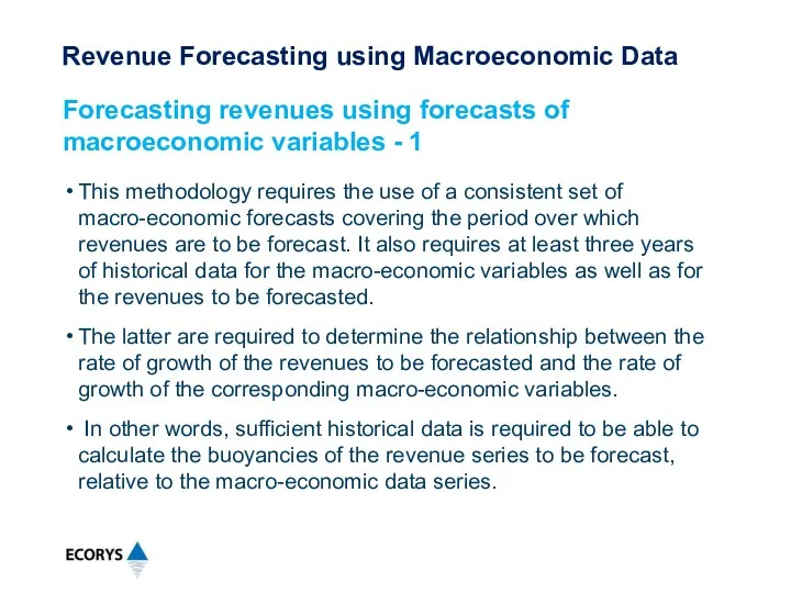
- 30. This methodology requires the use of a consistent set of macro-economic forecasts covering the period over
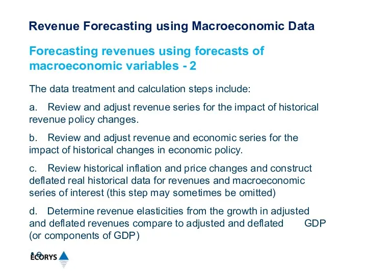
- 31. The data treatment and calculation steps include: a. Review and adjust revenue series for the impact
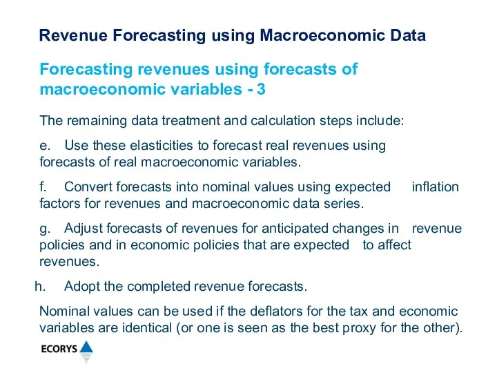
- 32. The remaining data treatment and calculation steps include: e. Use these elasticities to forecast real revenues
- 33. Using data from the Implementation of the State Budget, 2000-2014, it is possible to calculate the
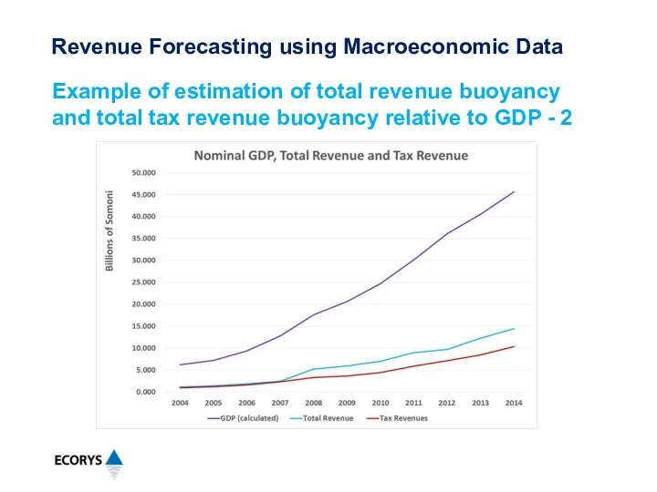
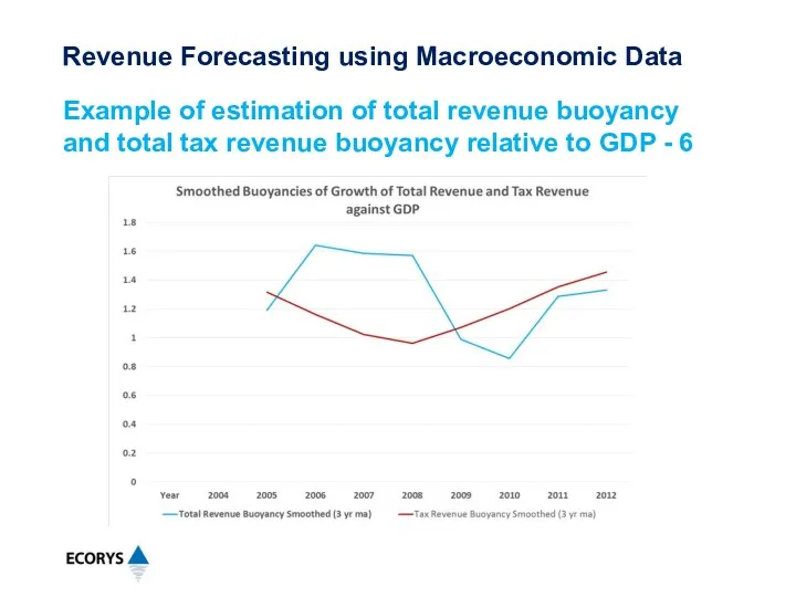
- 34. Example of estimation of total revenue buoyancy and total tax revenue buoyancy relative to GDP -
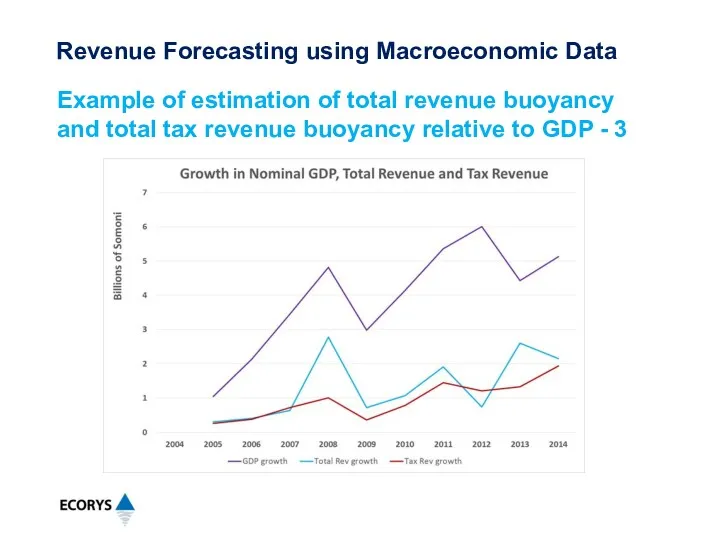
- 35. Example of estimation of total revenue buoyancy and total tax revenue buoyancy relative to GDP -
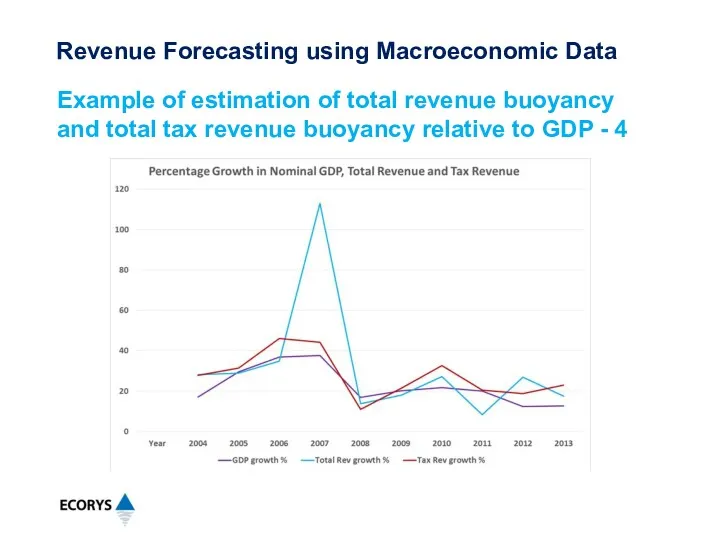
- 36. Example of estimation of total revenue buoyancy and total tax revenue buoyancy relative to GDP -
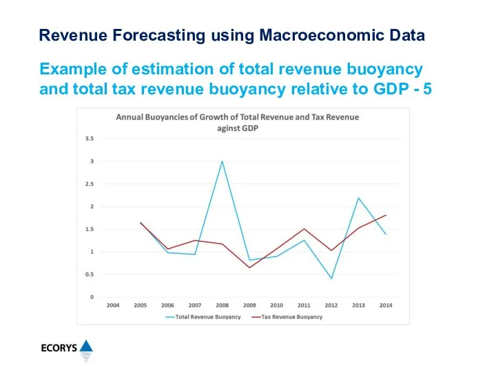
- 37. Example of estimation of total revenue buoyancy and total tax revenue buoyancy relative to GDP -
- 38. Example of estimation of total revenue buoyancy and total tax revenue buoyancy relative to GDP -
- 39. Because there is no policy related information available about the historical revenues, we can calculate only
- 40. The calculated results are Eb (total revenue to GDP) = 1.31 and Eb (tax revenue to
- 41. In summary, we expect total revenue in 2015 (and subsequently) to grow by 1.31 times the
- 43. Скачать презентацию
Revenue Forecasting - Day Three - Overview
Taxation and the Economy
Tax Elasticity
Revenue Forecasting - Day Three - Overview
Taxation and the Economy
Tax Elasticity
Revenue Forecasting – Session 1
Stylized flow of funds within the macro-economy
Macro-economic
Revenue Forecasting – Session 1
Stylized flow of funds within the macro-economy
Macro-economic
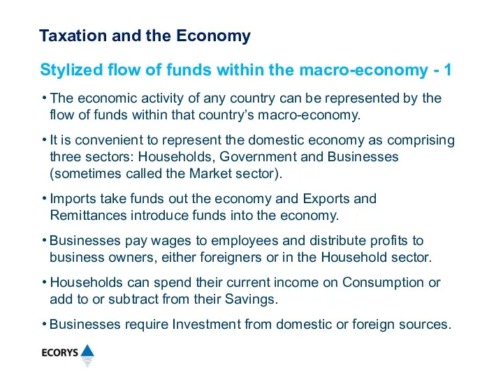
The economic activity of any country can be represented by the
The economic activity of any country can be represented by the
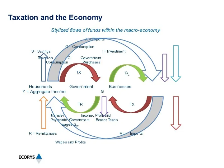
Stylized flows of funds within the macro-economy
X = Exports
Taxes
Stylized flows of funds within the macro-economy
X = Exports
Taxes
In a closed economy, business investment needs, I, must be funded
In a closed economy, business investment needs, I, must be funded
The circular flows of funding shown within the diagram are represented
The circular flows of funding shown within the diagram are represented
C is the aggregate consumption of goods and services within the
C is the aggregate consumption of goods and services within the
The government spends money on purchases of goods and services GC
The government spends money on purchases of goods and services GC
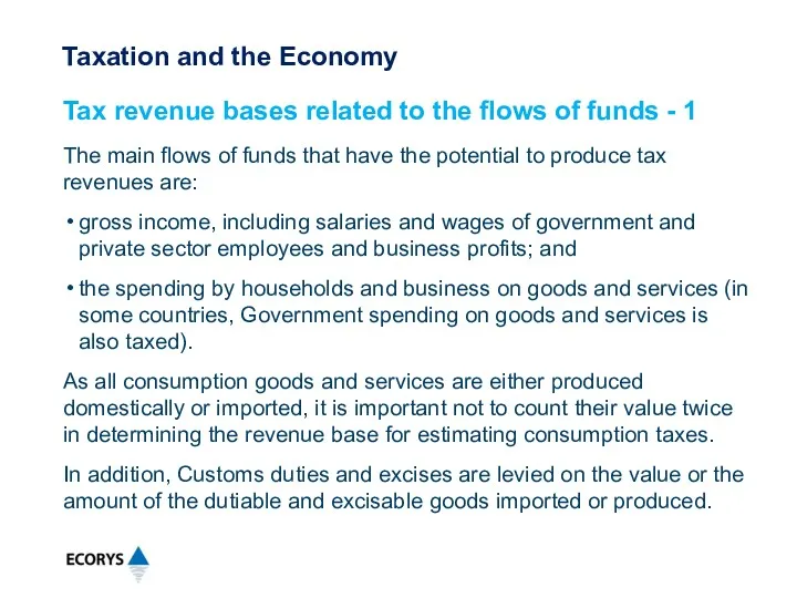
The main flows of funds that have the potential to produce
The main flows of funds that have the potential to produce
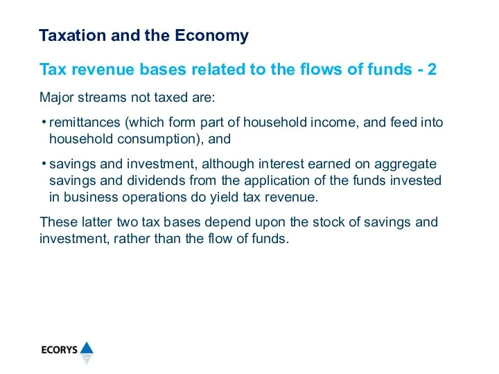
Major streams not taxed are:
remittances (which form part of household income,
Major streams not taxed are:
remittances (which form part of household income,
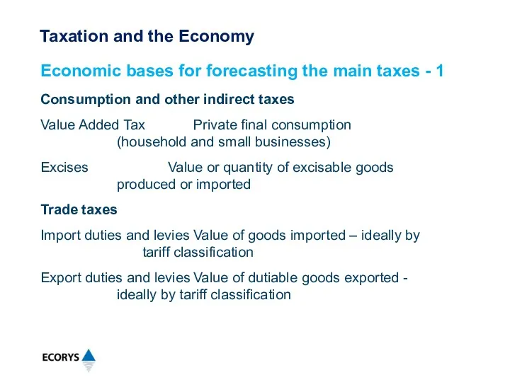
Consumption and other indirect taxes
Value Added Tax Private final consumption (household and
Consumption and other indirect taxes
Value Added Tax Private final consumption (household and
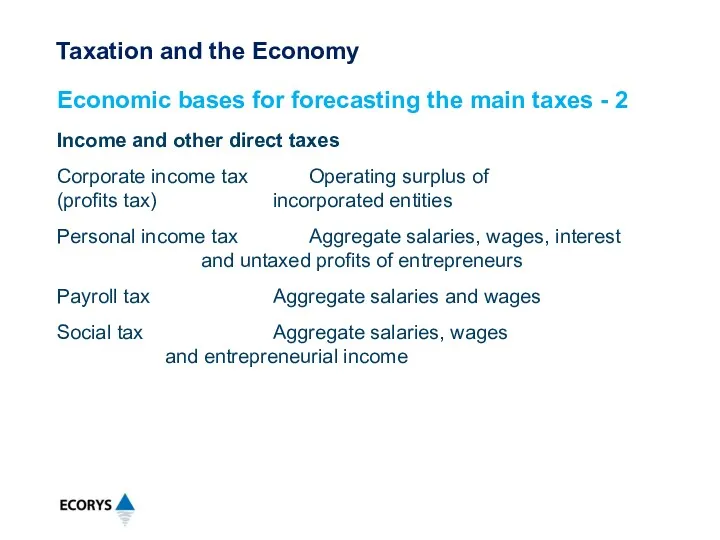
Income and other direct taxes
Corporate income tax Operating surplus of
(profits
Income and other direct taxes
Corporate income tax Operating surplus of
(profits
Revenue Forecasting – Session 2
Definitions of tax buoyancy and tax elasticity
Differences
Revenue Forecasting – Session 2
Definitions of tax buoyancy and tax elasticity
Differences
Tax Buoyancy
Tax buoyancy measures the total response of tax revenues to
Tax Buoyancy
Tax buoyancy measures the total response of tax revenues to
Tax Elasticity
Tax elasticity measures the pure response of tax revenues to
Tax Elasticity
Tax elasticity measures the pure response of tax revenues to
Tax buoyancy is the most appropriate measure when assessing the impact
Tax buoyancy is the most appropriate measure when assessing the impact
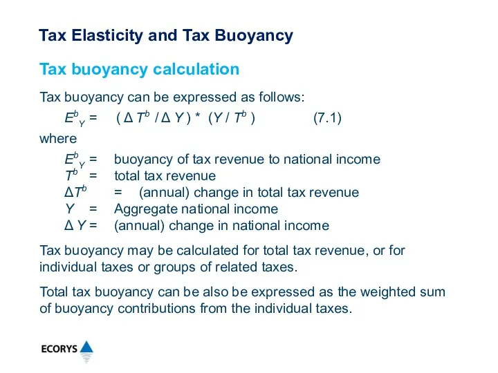
Tax buoyancy can be expressed as follows:
EbY = ( Δ Tb
Tax buoyancy can be expressed as follows:
EbY = ( Δ Tb
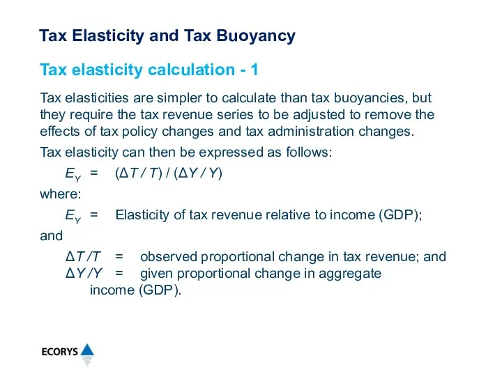
Tax elasticities are simpler to calculate than tax buoyancies, but they
Tax elasticities are simpler to calculate than tax buoyancies, but they
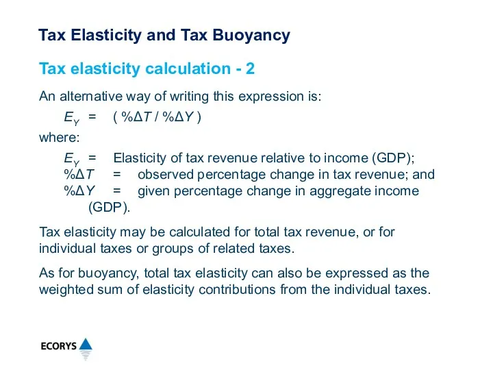
An alternative way of writing this expression is:
EY = ( %ΔT / %ΔY
An alternative way of writing this expression is:
EY = ( %ΔT / %ΔY
Each of the measures, Buoyancy and Elasticity, may have values less
Each of the measures, Buoyancy and Elasticity, may have values less
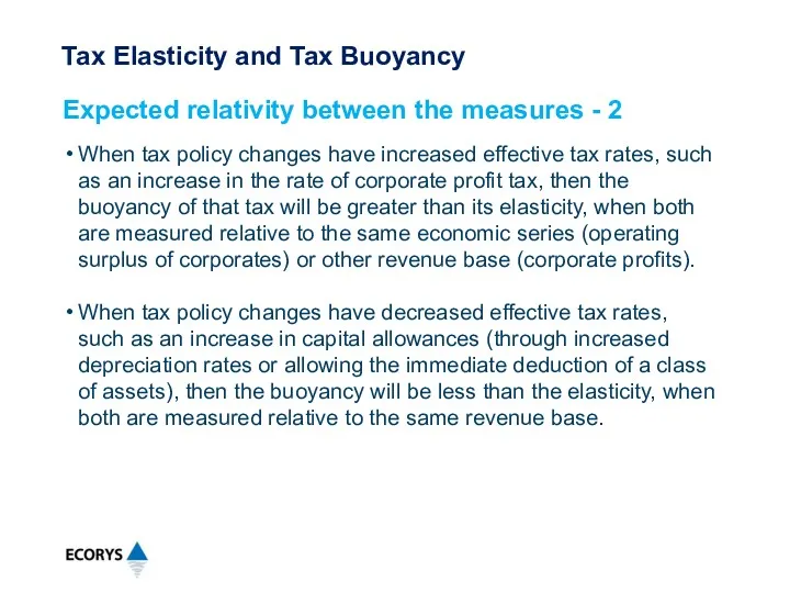
When tax policy changes have increased effective tax rates, such as
When tax policy changes have increased effective tax rates, such as
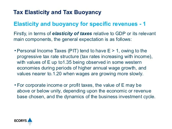
Firstly, in terms of elasticity of taxes relative to GDP or
Firstly, in terms of elasticity of taxes relative to GDP or
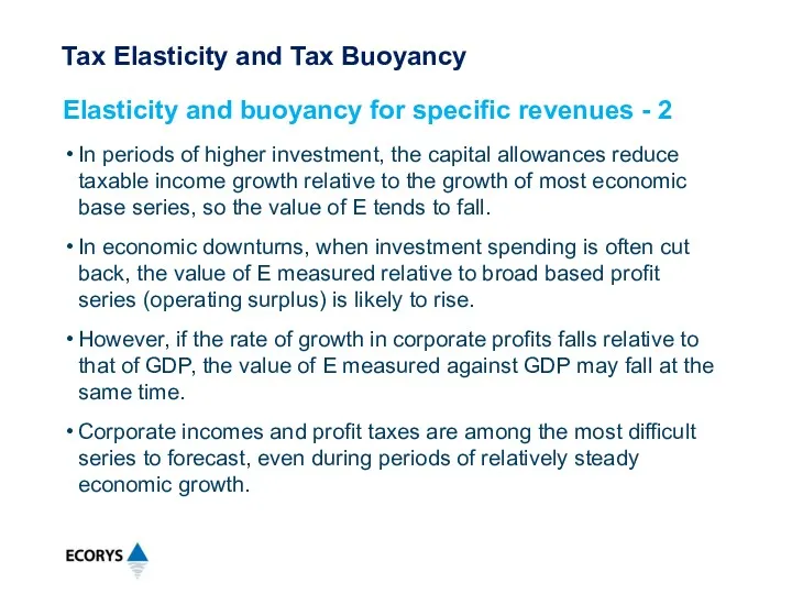
In periods of higher investment, the capital allowances reduce taxable income
In periods of higher investment, the capital allowances reduce taxable income
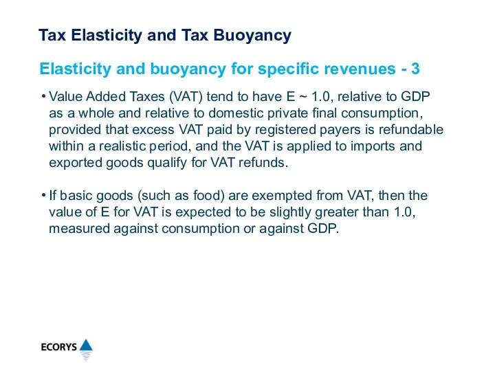
Value Added Taxes (VAT) tend to have E ~ 1.0, relative
Value Added Taxes (VAT) tend to have E ~ 1.0, relative
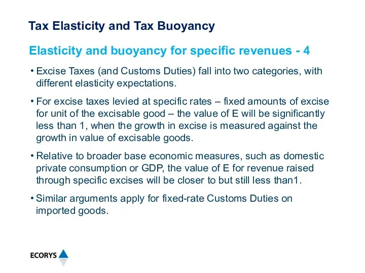
Excise Taxes (and Customs Duties) fall into two categories, with different
Excise Taxes (and Customs Duties) fall into two categories, with different
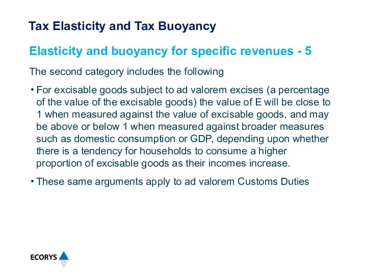
The second category includes the following
For excisable goods subject to ad
The second category includes the following
For excisable goods subject to ad
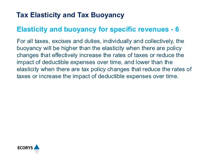
For all taxes, excises and duties, individually and collectively, the buoyancy
For all taxes, excises and duties, individually and collectively, the buoyancy
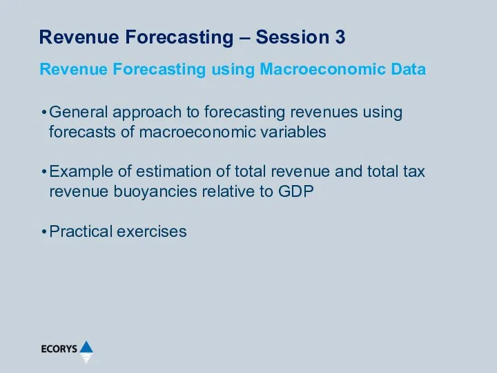
Revenue Forecasting – Session 3
General approach to forecasting revenues using forecasts
Revenue Forecasting – Session 3
General approach to forecasting revenues using forecasts
This methodology requires the use of a consistent set of macro-economic
This methodology requires the use of a consistent set of macro-economic
The data treatment and calculation steps include:
a. Review and adjust revenue series
The data treatment and calculation steps include:
a. Review and adjust revenue series
The remaining data treatment and calculation steps include:
e. Use these elasticities to
The remaining data treatment and calculation steps include:
e. Use these elasticities to
Using data from the Implementation of the State Budget, 2000-2014, it
Using data from the Implementation of the State Budget, 2000-2014, it
Example of estimation of total revenue buoyancy and total tax revenue
Example of estimation of total revenue buoyancy and total tax revenue
Example of estimation of total revenue buoyancy and total tax revenue
Example of estimation of total revenue buoyancy and total tax revenue
Example of estimation of total revenue buoyancy and total tax revenue
Example of estimation of total revenue buoyancy and total tax revenue
Example of estimation of total revenue buoyancy and total tax revenue
Example of estimation of total revenue buoyancy and total tax revenue
Example of estimation of total revenue buoyancy and total tax revenue
Example of estimation of total revenue buoyancy and total tax revenue
Because there is no policy related information available about the historical
Because there is no policy related information available about the historical
The calculated results are Eb (total revenue to GDP) = 1.31
The calculated results are Eb (total revenue to GDP) = 1.31
In summary, we expect total revenue in 2015 (and subsequently) to
In summary, we expect total revenue in 2015 (and subsequently) to
 Региональная экономика и управление. Целевые программы
 Инфляция и ее виды
 Конкуренция. Структура рынка. (9 класс)
 Цикличность экономического развития как закономерность макроэкономики. Безработица и инфляция. Лекция 8
 Ценности и потери
 Предмет экономики. Общественное производство
 Макроэкономика. Методология макроэкономики. (Тема 1)
 Краснодарский край
 Рынки факторов производства. Тема 10
 Капитальное строительство как инвестиционный процесс
 “Камолот” ЁИҲ “Камолот стипендиясига номзод
 Макроэкономикалық тепе-теңдік
 Мировое хозяйство и международная торговля. (Обществознание. 8 класс)
 Международная экономическая интеграция (часть 2)
 Чистая монополия. Показатель А. Лернера. Индекс Херфиндаля-Хиршмана. Ценовая дискриминация
 Хозяйство США. Роль США в мировом хозяйстве
 Рыночные отношения в экономике. 11 класс
 Новая экономическая политика НЭП. 11 класс
 Теории пространственного размещения и ядрообразовния
 Услуги салонов красоты. Анализ рынка
 World economics: Modern Factors of Economic Growth and Economic Development
 Эколого-экономическая политика России
 Өндіріс теориясі
 Қазақстадағы шетел мұнай компанялары
 Особенности социальноэкономического развития мировой экономики в 1950-1990-е гг
 Вход, выход и формирование рынков. Концепции современной теории отраслевых рынков
 Презентация Спрос и предложение 10 класс
 Общественное производство. Экономические системы и отношения