- Unemployment rate

Содержание
- 2. Let’s review our voyage to date: We have analyzed: Measuring economic activity Aggregate production functions and
- 3. What picture do you have in mind when you think of business cycles? “Note that the
- 4. Understanding business cycles Major elements of cycles short-period (1-3 yr) erratic fluctuations in output pro-cyclical movements
- 5. Output gap and recessions
- 6. Unemployment and recessions
- 7. Unemployment and vacancies (2000-2010)
- 8. So what’s the big problem for economics? Many economists worry that there are no firm “microeconomic
- 10. This has been the approach up to now.
- 11. We now move to a different set of assumptions/observations
- 12. Major approaches to business cycles Classical: market clearing: supply-side cycles with vertical AS curve: Real business
- 13. Real output (Y) Expenditures C+I+G+NX Y* E* Equilibrium output Keynesian Cross Diagram: Output where planned expenditure
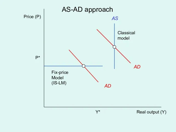
- 14. Real output (Y) Price (P) AD AS Y* P* Classical model Fix-price Model (IS-LM) AS-AD approach
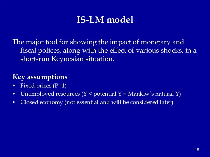
- 15. IS-LM model The major tool for showing the impact of monetary and fiscal polices, along with
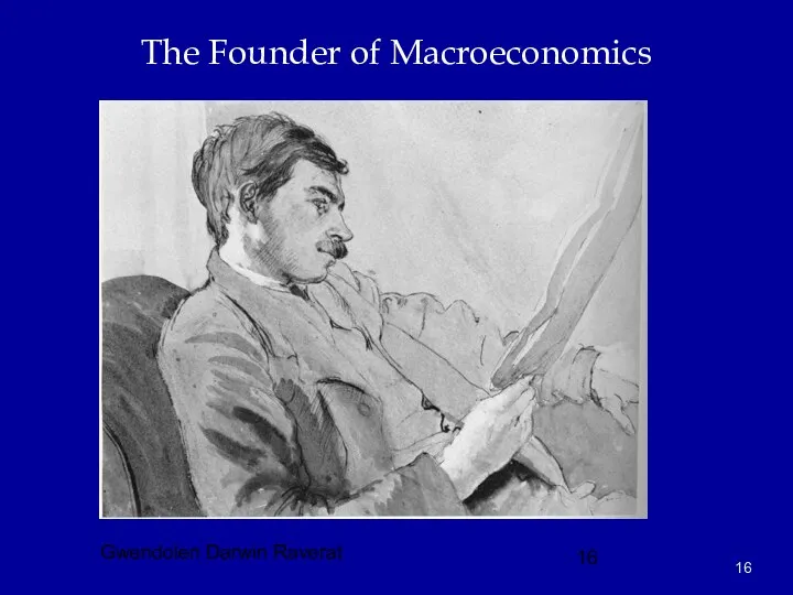
- 16. The Founder of Macroeconomics Gwendolen Darwin Raverat
- 17. Keynes on Why macroeconomics is difficult or Why the models are so confusing! Professor Planck, of
- 19. Where are we? We are now attempting to understand the basic features of business cycles. Aggregate
- 20. IS curve (expenditures) Basic idea: describes equilibrium in goods market Finds Y where planned I =
- 21. which gives the IS curve: Y = a - bT0 + G0 + I0 - dr
- 22. LM curve (financial markets) The LM curve represents equilibrium in financial markets, or where the supply
- 23. Summary of IS-LM Y ≡ C + I + G C = a + b(Y-T) T
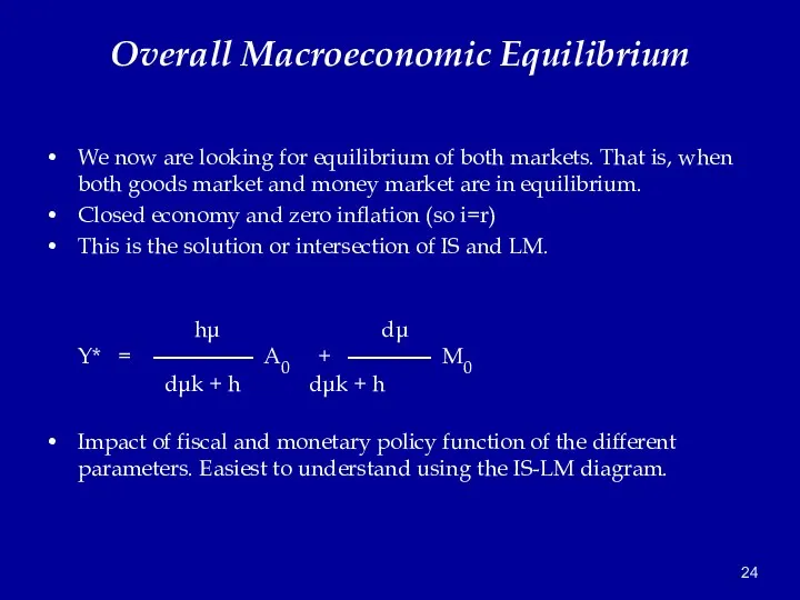
- 24. Overall Macroeconomic Equilibrium We now are looking for equilibrium of both markets. That is, when both
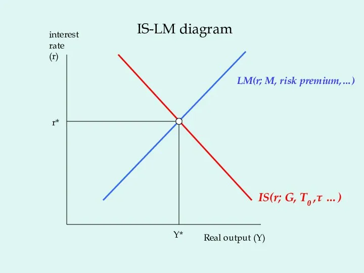
- 25. Real output (Y) interest rate (r) IS(r; G, T0 ,τ …) LM(r; M, risk premium,…) Y*
- 26. SOME BASICS OF THE IS-LM MODEL Have two major kinds of shocks in business cycles: IS:
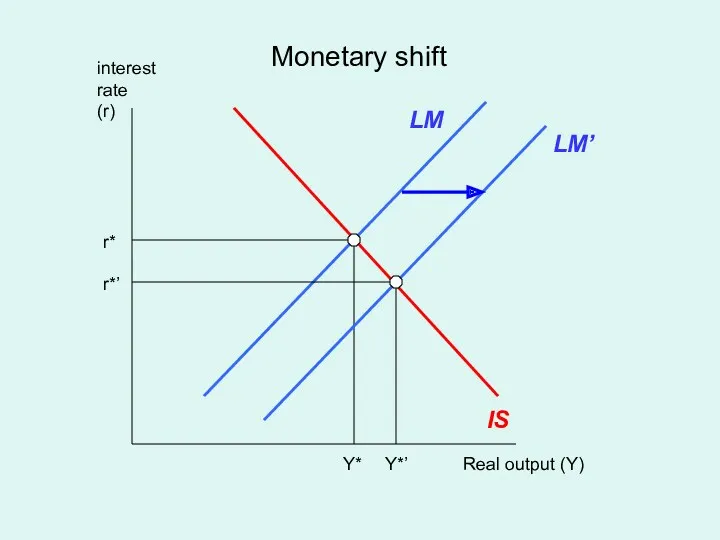
- 27. Now several interesting cases Case 1. A change in monetary policy Note: by a monetary policy,
- 28. Real output (Y) interest rate (r) IS LM Y* r* Monetary shift LM’ Y*’ r*’
- 29. More on financial issues… Case 1A. A monetary crisis that increases risk premiums - This important
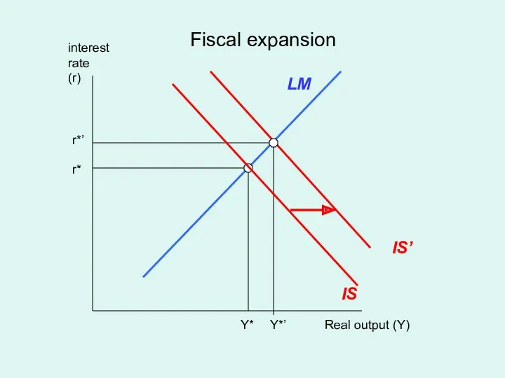
- 30. Case 2. What are the effects of fiscal policy? A fiscal policy shift is change in
- 31. Real output (Y) interest rate (r) IS LM Y* r* Fiscal expansion Y*’ r*’ IS’
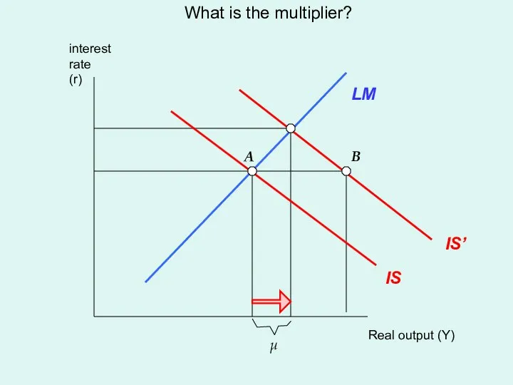
- 32. Real output (Y) interest rate (r) IS LM What is the multiplier? IS’ μ A B
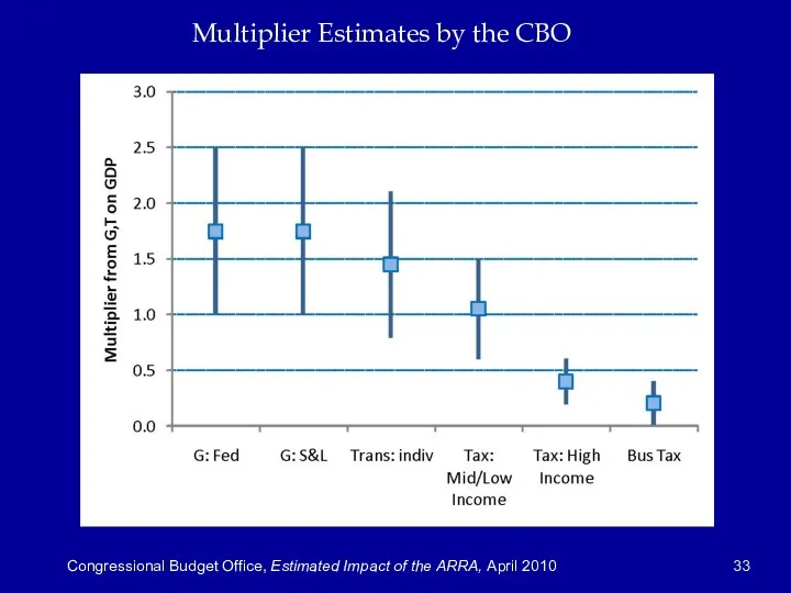
- 33. Multiplier Estimates by the CBO Congressional Budget Office, Estimated Impact of the ARRA, April 2010
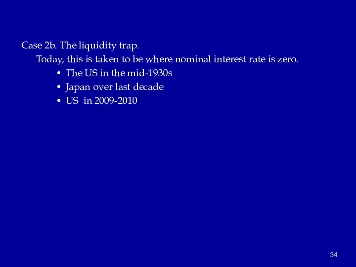
- 34. Case 2b. The liquidity trap. Today, this is taken to be where nominal interest rate is
- 35. Liquidity trap in US in Great Depression
- 36. Japan short-term interest rates, 1994-2006 Liquidity trap from 1999 to early 2006
- 37. US today Policy has hit the “zero lower bound” this year.
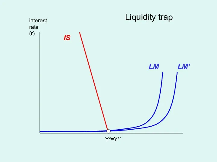
- 38. interest rate (r) IS Y*=Y*’ Liquidity trap LM LM’
- 39. Heavy hitters in the Obama administration Regulation: Cass Sunstein Departed budget: Peter Orszag Economics czar Larry
- 40. Can you see why macroeconomists emphasize the importance of fiscal policy in the current environment? “Our
- 41. The monetarist regime: "Only money matters for output determination.“ (Milton Friedman). We can go back to
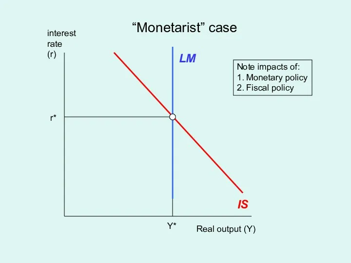
- 42. Real output (Y) interest rate (r) IS LM Y* r* “Monetarist” case Note impacts of: 1.
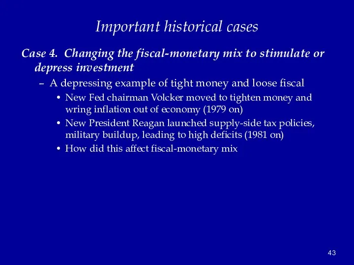
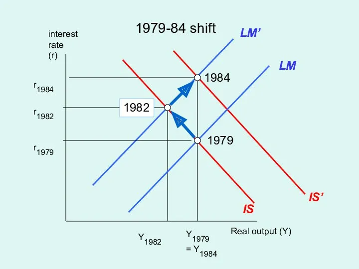
- 43. Important historical cases Case 4. Changing the fiscal-monetary mix to stimulate or depress investment A depressing
- 44. Real output (Y) interest rate (r) IS LM 1979-84 shift LM’ r1979 Y1979 Y1982 = Y1984
- 45. Important historical cases Pro-growth policies The opposite would be to tighten fiscal policies and loosen monetary
- 47. Скачать презентацию
Let’s review our voyage to date:
We have analyzed:
Measuring economic activity
Aggregate production
Let’s review our voyage to date:
We have analyzed:
Measuring economic activity
Aggregate production
What picture do you have in mind when you think of
What picture do you have in mind when you think of
Understanding business cycles
Major elements of cycles
short-period (1-3 yr) erratic fluctuations in
Understanding business cycles
Major elements of cycles
short-period (1-3 yr) erratic fluctuations in
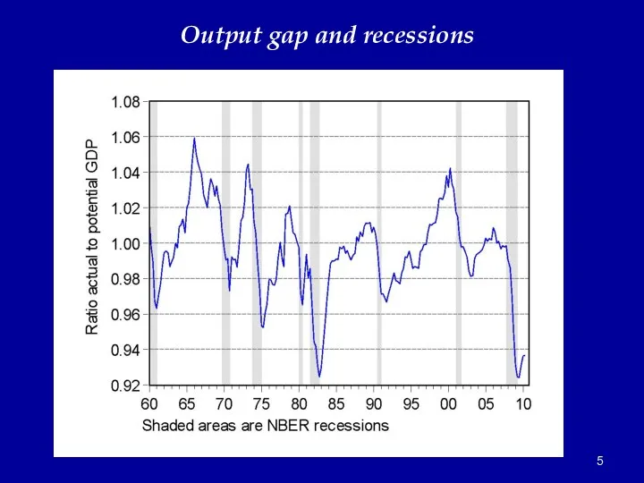
Output gap and recessions
Output gap and recessions
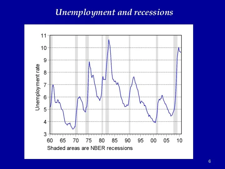
Unemployment and recessions
Unemployment and recessions
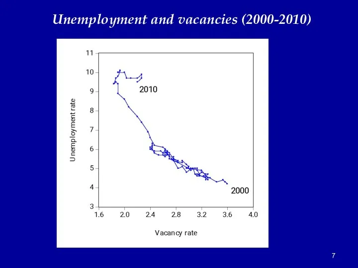
Unemployment and vacancies (2000-2010)
Unemployment and vacancies (2000-2010)
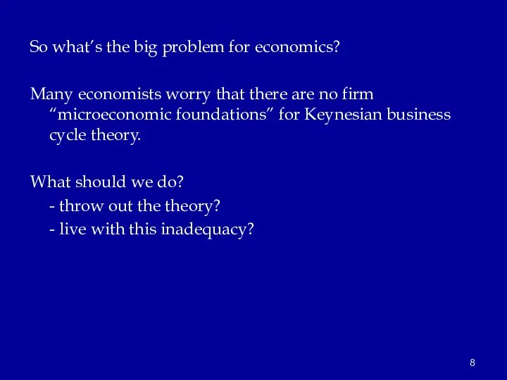
So what’s the big problem for economics?
Many economists worry that there
So what’s the big problem for economics?
Many economists worry that there
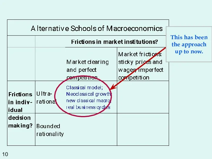
This has been the approach up to now.
This has been the approach up to now.
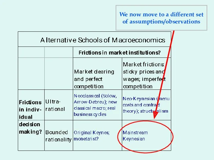
We now move to a different set of assumptions/observations
We now move to a different set of assumptions/observations
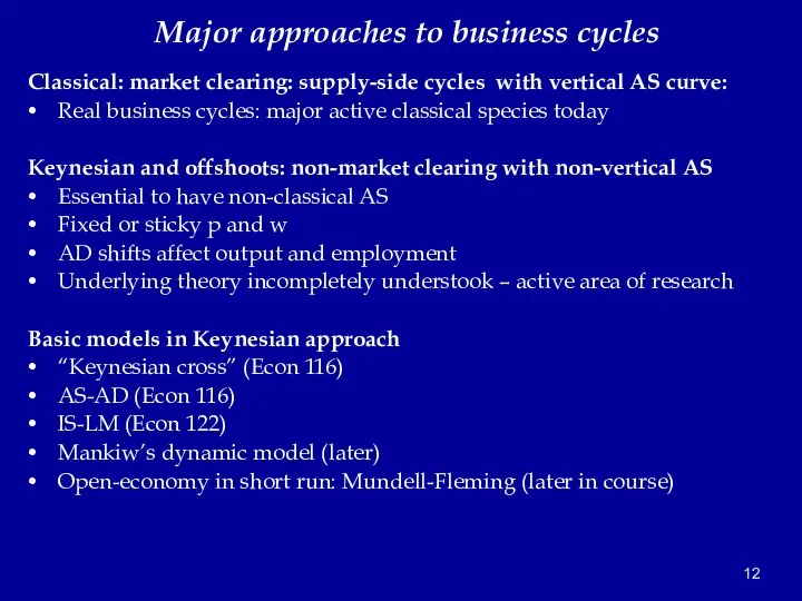
Major approaches to business cycles
Classical: market clearing: supply-side cycles with vertical
Major approaches to business cycles
Classical: market clearing: supply-side cycles with vertical
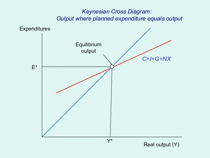
Real output (Y)
Expenditures
C+I+G+NX
Y*
E*
Equilibrium
output
Keynesian Cross Diagram:
Output where planned expenditure
Real output (Y)
Expenditures
C+I+G+NX
Y*
E*
Equilibrium
output
Keynesian Cross Diagram:
Output where planned expenditure
Real output (Y)
Price (P)
AD
AS
Y*
P*
Classical
model
Fix-price
Model
(IS-LM)
AS-AD approach
AD
Real output (Y)
Price (P)
AD
AS
Y*
P*
Classical
model
Fix-price
Model
(IS-LM)
AS-AD approach
AD
IS-LM model
The major tool for showing the impact of monetary and
IS-LM model
The major tool for showing the impact of monetary and
The Founder of Macroeconomics
Gwendolen Darwin Raverat
The Founder of Macroeconomics
Gwendolen Darwin Raverat

Keynes on Why macroeconomics is difficult
or
Why the models are so confusing!
Professor
Keynes on Why macroeconomics is difficult
or
Why the models are so confusing!
Professor
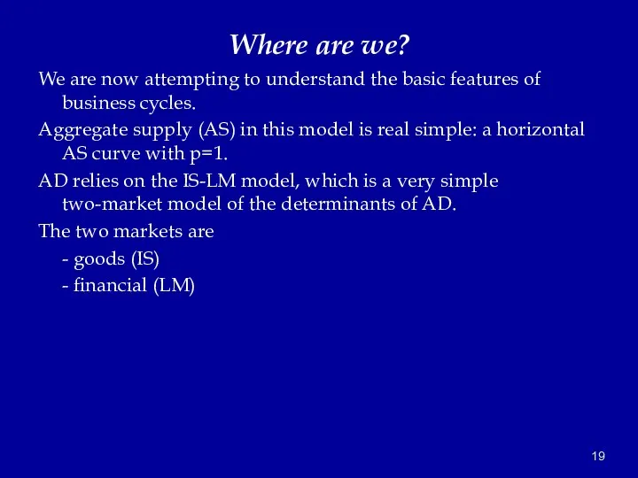
Where are we?
We are now attempting to understand the basic features
Where are we?
We are now attempting to understand the basic features
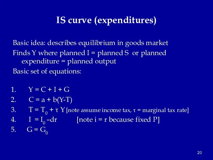
IS curve (expenditures)
Basic idea: describes equilibrium in goods market
Finds Y where
IS curve (expenditures)
Basic idea: describes equilibrium in goods market
Finds Y where
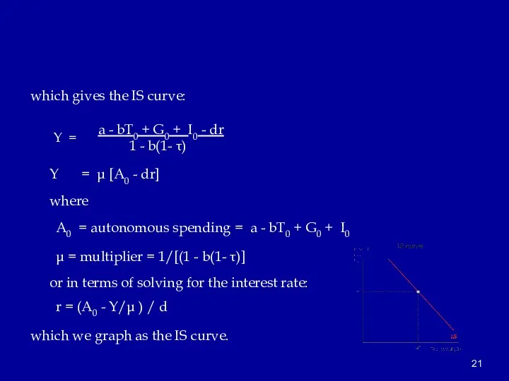
which gives the IS curve:
Y = a - bT0 +
which gives the IS curve:
Y = a - bT0 +
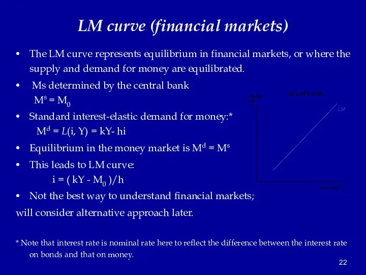
LM curve (financial markets)
The LM curve represents equilibrium in financial markets,
LM curve (financial markets)
The LM curve represents equilibrium in financial markets,
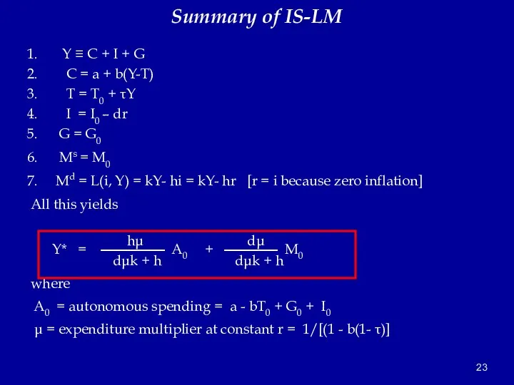
Summary of IS-LM
Y ≡ C + I + G
C
Summary of IS-LM
Y ≡ C + I + G
C
Overall Macroeconomic Equilibrium
We now are looking for equilibrium of both markets.
Overall Macroeconomic Equilibrium
We now are looking for equilibrium of both markets.
Real output (Y)
interest
rate
(r)
IS(r; G, T0 ,τ …)
LM(r; M, risk premium,…)
Y*
r*
IS-LM diagram
Real output (Y)
interest
rate
(r)
IS(r; G, T0 ,τ …)
LM(r; M, risk premium,…)
Y*
r*
IS-LM diagram
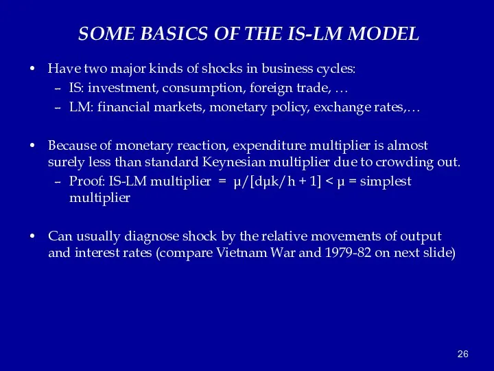
SOME BASICS OF THE IS-LM MODEL
Have two major kinds of
SOME BASICS OF THE IS-LM MODEL
Have two major kinds of
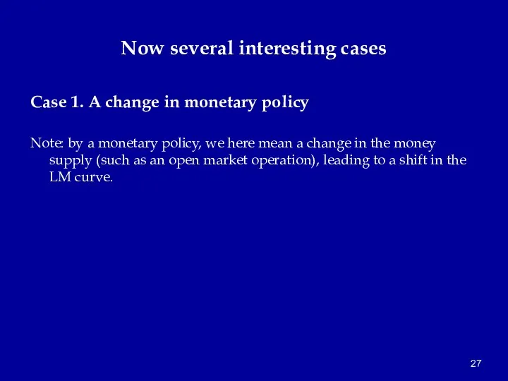
Now several interesting cases
Case 1. A change in monetary policy
Note: by
Now several interesting cases
Case 1. A change in monetary policy
Note: by
Real output (Y)
interest
rate
(r)
IS
LM
Y*
r*
Monetary shift
LM’
Y*’
r*’
Real output (Y)
interest
rate
(r)
IS
LM
Y*
r*
Monetary shift
LM’
Y*’
r*’
More on financial issues…
Case 1A. A monetary crisis that increases risk
More on financial issues…
Case 1A. A monetary crisis that increases risk
Case 2. What are the effects of fiscal policy?
A fiscal policy
Case 2. What are the effects of fiscal policy?
A fiscal policy
Real output (Y)
interest
rate
(r)
IS
LM
Y*
r*
Fiscal expansion
Y*’
r*’
IS’
Real output (Y)
interest
rate
(r)
IS
LM
Y*
r*
Fiscal expansion
Y*’
r*’
IS’
Real output (Y)
interest
rate
(r)
IS
LM
What is the multiplier?
IS’
μ
A
B
Real output (Y)
interest
rate
(r)
IS
LM
What is the multiplier?
IS’
μ
A
B
Multiplier Estimates by the CBO
Congressional Budget Office, Estimated Impact of the
Multiplier Estimates by the CBO
Congressional Budget Office, Estimated Impact of the
Case 2b. The liquidity trap.
Today, this is taken to be
Today, this is taken to be
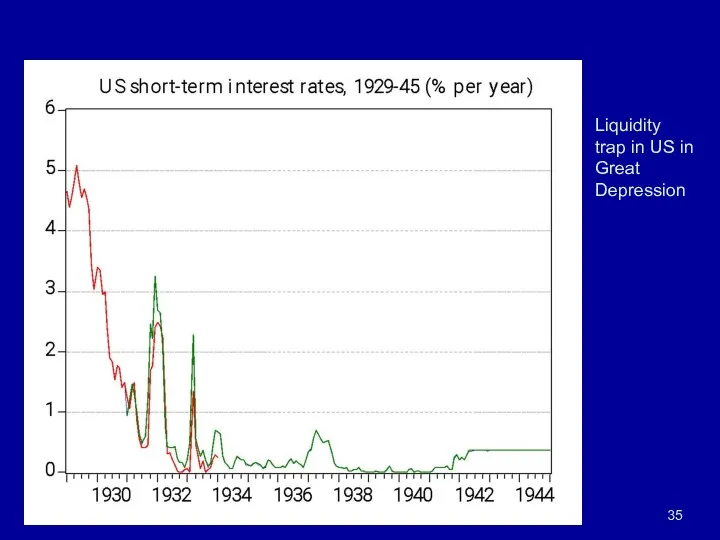
Liquidity trap in US in Great Depression
Liquidity trap in US in Great Depression
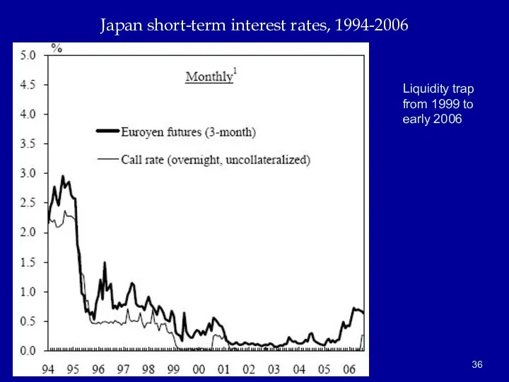
Japan short-term interest rates, 1994-2006
Liquidity trap from 1999 to early 2006
Japan short-term interest rates, 1994-2006
Liquidity trap from 1999 to early 2006
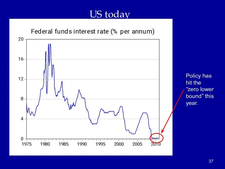
US today
Policy has hit the “zero lower bound” this year.
US today
Policy has hit the “zero lower bound” this year.
interest
rate
(r)
IS
Y*=Y*’
Liquidity trap
LM
LM’
interest
rate
(r)
IS
Y*=Y*’
Liquidity trap
LM
LM’

Heavy hitters in the Obama administration
Regulation: Cass Sunstein
Departed budget: Peter Orszag
Economics
Heavy hitters in the Obama administration
Regulation: Cass Sunstein
Departed budget: Peter Orszag
Economics
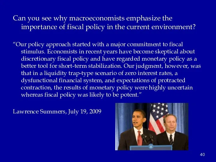
Can you see why macroeconomists emphasize the importance of fiscal policy
Can you see why macroeconomists emphasize the importance of fiscal policy
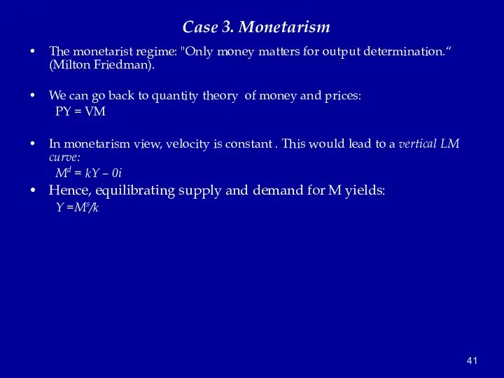
The monetarist regime: "Only money matters for output determination.“ (Milton Friedman).
We
The monetarist regime: "Only money matters for output determination.“ (Milton Friedman).
We
Real output (Y)
interest
rate
(r)
IS
LM
Y*
r*
“Monetarist” case
Note impacts of:
1. Monetary policy
2. Fiscal policy
Real output (Y)
interest
rate
(r)
IS
LM
Y*
r*
“Monetarist” case
Note impacts of:
1. Monetary policy
2. Fiscal policy
Important historical cases
Case 4. Changing the fiscal-monetary mix to stimulate or
Important historical cases
Case 4. Changing the fiscal-monetary mix to stimulate or
Real output (Y)
interest
rate
(r)
IS
LM
1979-84 shift
LM’
r1979
Y1979
Y1982
= Y1984
r1982
r1984
IS’
1984
1979
1982
Real output (Y)
interest
rate
(r)
IS
LM
1979-84 shift
LM’
r1979
Y1979
Y1982
= Y1984
r1982
r1984
IS’
1984
1979
1982
Important historical cases
Pro-growth policies
The opposite would be to tighten fiscal policies
Important historical cases
Pro-growth policies
The opposite would be to tighten fiscal policies
 Промышленность РСО Алании. Лабораторная работа №4
 Анализ социально-экономических показателей тверской области
 Своя игра. Обществознание
 Основы внутрифирменного планирования
 Организационное проектирование
 World Tourism Market. Introduction to the market and international tourism
 Теория потребительского поведения
 Ефективність виробництва
 Обеспечение экономической состоятельности организации
 Сегмент упаковки в экономике замкнутого цикла
 Қазақстан тәуелсіздігі , ел басы , 2030 стратегиясы
 Cистема основных счетов СНС
 Вектор развития внешнеэкономической деятельности России в условиях экономических санкций
 Человек в экономике
 Многообразие рынков
 Рынок
Рынок The Economist: The Work of Calculation
 Внешнеторговые взаимоотношения Российской Федерации и Европейского союза. Таможенный аспект
 Проблема терроризма в России. Бесланская трагедия
 Конкурентоспособность предприятий сферы услуг в условиях глобализации экономики
 Экономика. Семейный бюджет
 Историческая школа Германии. Институционализм. Условия появления институционализма. (Занятие 8)
 Безработица и инфляция как проявления экономической нестабильности
 Налоги
 Экономика. Учебники из ЭБС
 Модели потребления, сбережения, инвестиций
 Научно-техническая революция и мировое хозяйство. Лекция 4
 Собственность и ее место в экономической системе. Модели экономических систем. Рыночная экономика