- Course of lectures Contemporary Physics: Part1

Содержание
- 2. Figure 4.1. Two particles interact with each other. According to Newton’s third law, we must have
- 3. The linear momentum of a particle or an object that can be modeled as a particle
- 4. As you can see from its definition, the concept of momentum provides a quantitative distinction between
- 5. Using Newton’s second law of motion, we can relate the linear momentum of a particle to
- 6. Using the definition of momentum, Equation 4.1 can be written where p1i and p2i are the
- 7. This result, known as the law of conservation of linear momentum, can be extended to any
- 8. The momentum of a particle changes if a net force acts on the particle. According to
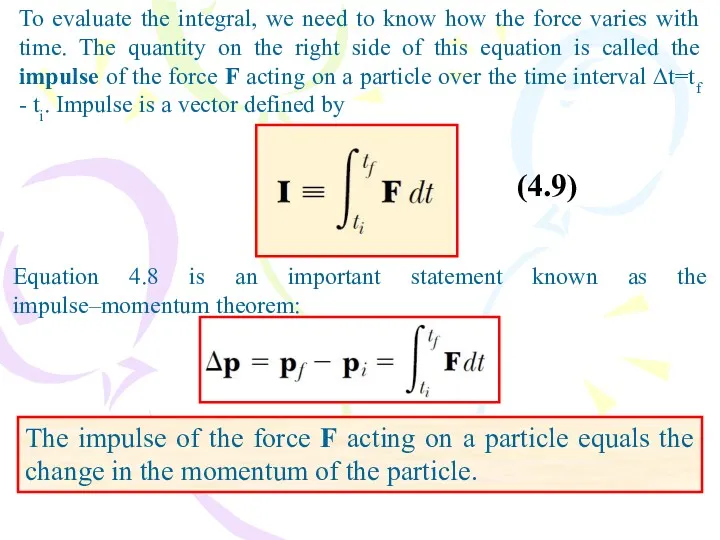
- 9. (4.9) To evaluate the integral, we need to know how the force varies with time. The
- 10. The direction of the impulse vector is the same as the direction of the change in
- 11. Because the force imparting an impulse can generally vary in time, it is convenient to define
- 12. We use the term collision to represent an event during which two particles come close to
- 13. The total momentum of an isolated system just before a collision equals the total momentum of
- 14. An inelastic collision is one in which the total kinetic energy of the system is not
- 15. Figure 4.4 Schematic representation of a perfectly inelastic head-on collision between two particles: (a) before collision
- 16. Figure 4.5 Schematic representation of an elastic head-on collision between two particles: (a) before collision and
- 17. Next, let us separate the terms containing m1 and m2 in Equation 4.15 to obtain (4.17)
- 18. Suppose that the masses and initial velocities of both particles are known. (4.20) (4.21) Let us
- 19. If particle 2 is initially at rest, then v2i = 0, and Equations 4.20 and 4.21
- 20. The momentum of a system of two particles is conserved when the system is isolated. For
- 21. Figure 4.6 An elastic glancing collision between two particles. glancing collision (4.25) (4.24)
- 22. (4.26) If the collision is elastic, we can also use Equation 4.16 (conservation of kinetic energy)
- 23. Figure 4.7 Two particles of unequal mass are connected by a light, rigid rod. (a) The
- 24. Figure 4.8 The center of mass of two particles of unequal mass on the x axis
- 25. (4.30) Figure 4.9 An extended object can be considered to be a distribution of small elements
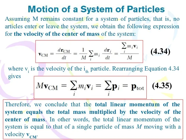
- 26. Assuming M remains constant for a system of particles, that is, no articles enter or leave
- 27. If we now differentiate Equation 4.34 with respect to time, we obtain the acceleration of the
- 28. That is, the net external force on a system of particles equals the total mass of
- 29. The angular position of the rigid object is the angle θ between this reference line on
- 30. Rotation of a Rigid Object About a Fixed Axis Figure 5.2 A particle on a rotating
- 31. The average angular acceleration The instantaneous angular acceleration When a rigid object is rotating about a
- 32. Direction for angular speed and angular acceleration Figure 5.3 The right-hand rule for determining the direction
- 33. Rotational Kinematics: Rotational Motion with Constant Angular Acceleration (5.6) is the angular speed of the rigid
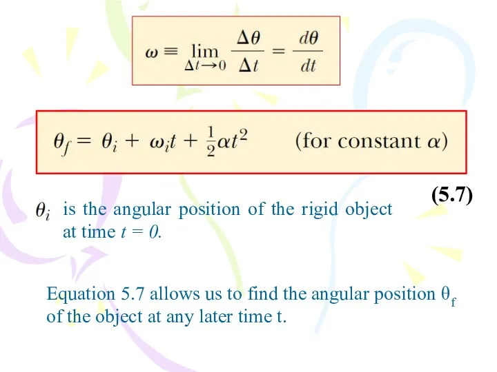
- 34. (5.7) is the angular position of the rigid object at time t = 0. Equation 5.7
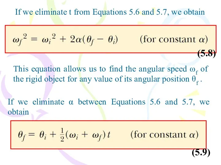
- 35. If we eliminate t from Equations 5.6 and 5.7, we obtain This equation allows us to
- 36. Table 5.1
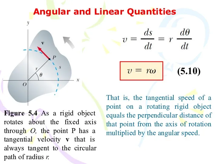
- 37. Angular and Linear Quantities Figure 5.4 As a rigid object rotates about the fixed axis through
- 38. We can relate the angular acceleration of the rotating rigid object to the tangential acceleration of
- 39. Figure 5.5 As a rigid object rotates about a fixed axis through O, the point P
- 40. Rotational Kinetic Energy Figure 10.7 A rigid object rotating about the z axis with angular speed
- 41. We simplify this expression by defining the quantity in parentheses as the moment of inertia I:
- 42. Calculation of Moments of Inertia (5.17)
- 43. Table 5.2
- 45. Torque Figure 5.8 The force F has a greater rotating tendency about O as F increases
- 46. Figure 5.9 The force F1 tends to rotate the object counterclockwise about O, and F2 tends
- 47. Relationship Between Torque and Angular Acceleration Figure 5.10 A particle rotating in a circle under the
- 48. The torque acting on the particle is proportional to its angular acceleration, and the proportionality constant
- 49. Figure 5.11 A rigid object rotating about an axis through O.
- 50. Although each mass element of the rigid object may have a different linear acceleration at ,
- 51. Work, Power, and Energy in Rotational Motion Figure 5.12 A rigid object rotates about an axis
- 52. The rate at which work is being done by F as the object rotates about the
- 53. (5.24)
- 54. That is, the work–kinetic energy theorem for rotational motion states that the net work done by
- 55. Table 5.3
- 56. Rolling Motion of a Rigid Object Figure 5.13 For pure rolling motion, as the cylinder rotates
- 57. Figure 5.14 All points on a rolling object move in a direction perpendicular to an axis
- 58. Figure 5.15 The motion of a rolling object can be modeled as a combination of pure
- 59. Find v1f and v2f. Quiz Figure 4.5 Schematic representation of an elastic head-on collision between two
- 61. Скачать презентацию
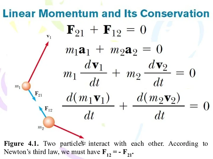
Figure 4.1. Two particles interact with each other. According to Newton’s
Figure 4.1. Two particles interact with each other. According to Newton’s
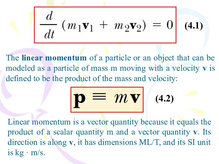
The linear momentum of a particle or an object that can
The linear momentum of a particle or an object that can
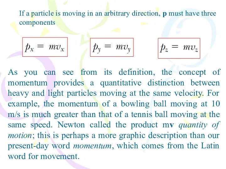
As you can see from its definition, the concept of momentum
As you can see from its definition, the concept of momentum
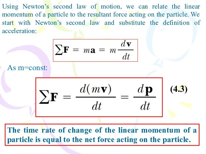
Using Newton’s second law of motion, we can relate the linear
Using Newton’s second law of motion, we can relate the linear
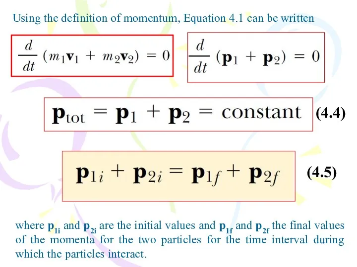
Using the definition of momentum, Equation 4.1 can be written
where p1i
Using the definition of momentum, Equation 4.1 can be written
where p1i
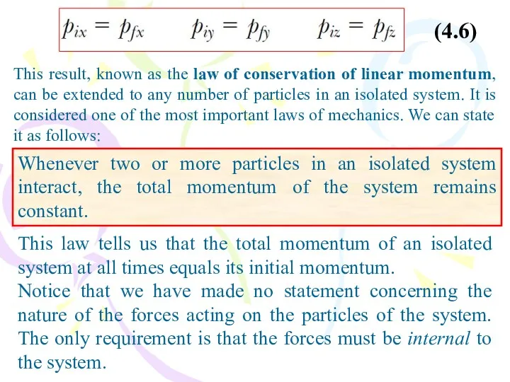
This result, known as the law of conservation of linear momentum,
This result, known as the law of conservation of linear momentum,
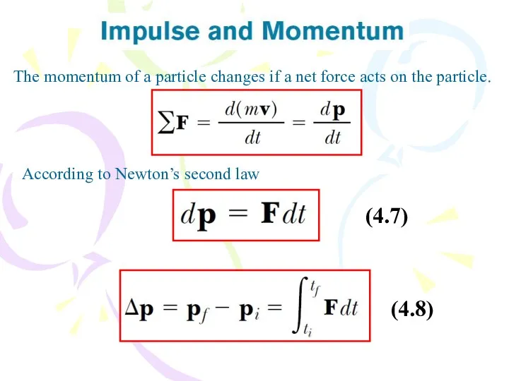
The momentum of a particle changes if a net force acts
The momentum of a particle changes if a net force acts
(4.9)
To evaluate the integral, we need to know how the force
(4.9)
To evaluate the integral, we need to know how the force
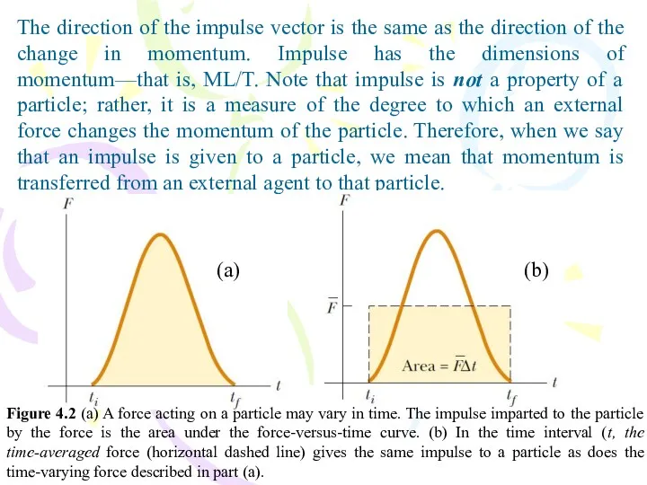
The direction of the impulse vector is the same as the
The direction of the impulse vector is the same as the
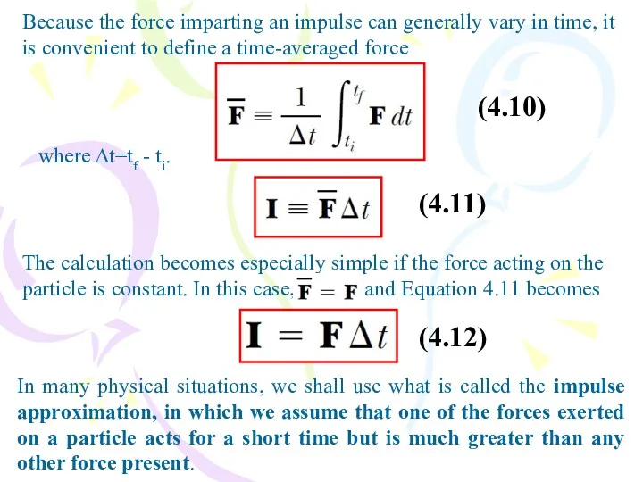
Because the force imparting an impulse can generally vary in time,
Because the force imparting an impulse can generally vary in time,
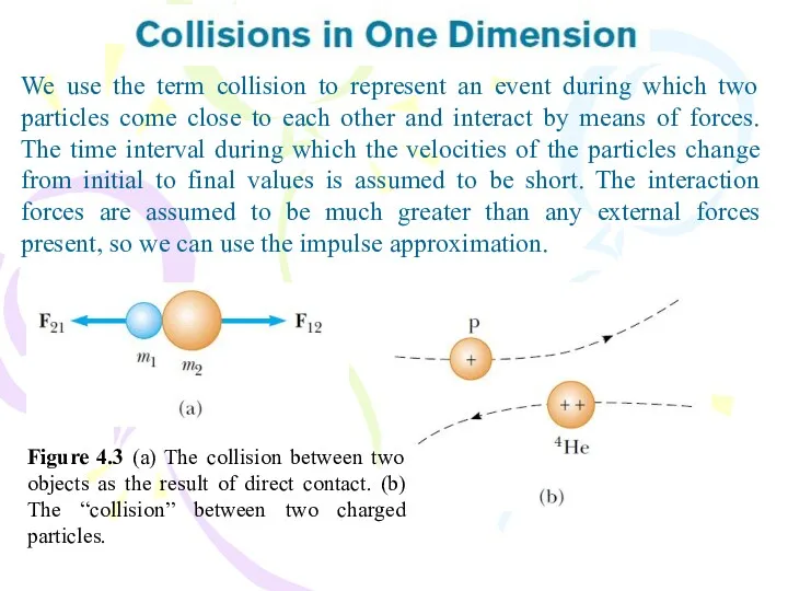
We use the term collision to represent an event during which
We use the term collision to represent an event during which
The total momentum of an isolated system just before a collision
The total momentum of an isolated system just before a collision
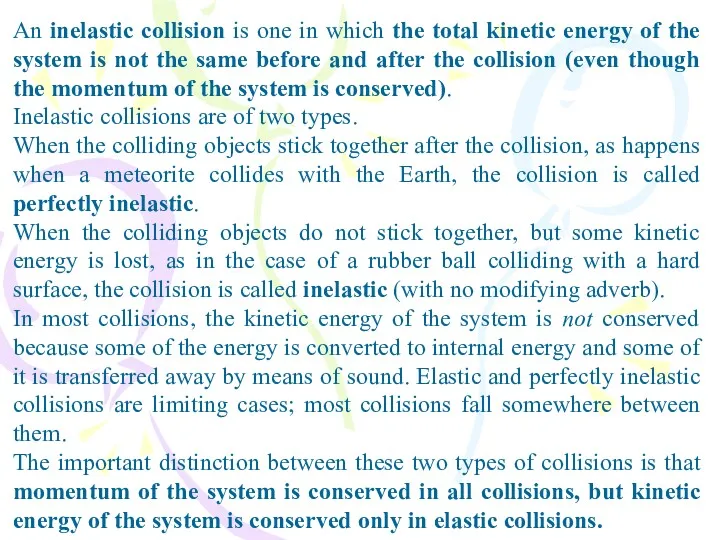
An inelastic collision is one in which the total kinetic energy
An inelastic collision is one in which the total kinetic energy
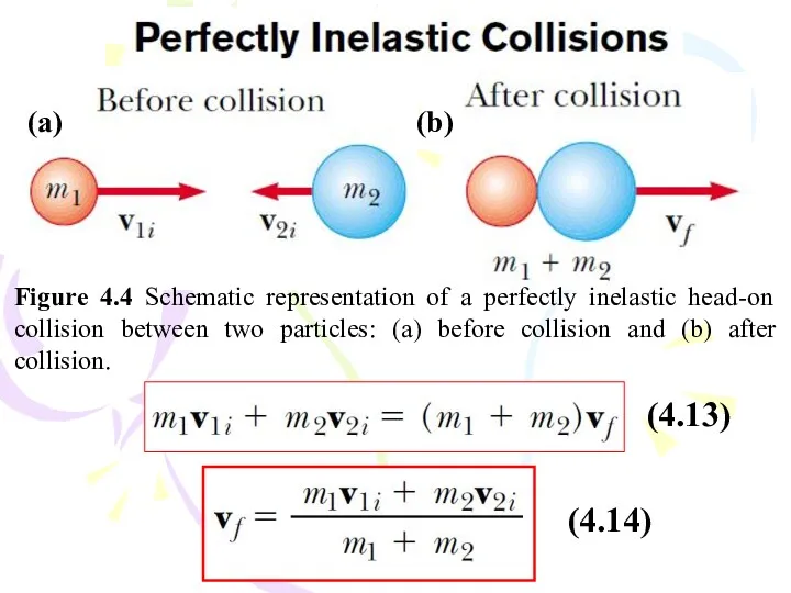
Figure 4.4 Schematic representation of a perfectly inelastic head-on collision between
Figure 4.4 Schematic representation of a perfectly inelastic head-on collision between
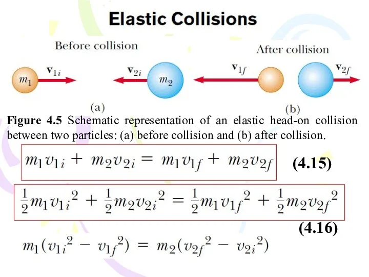
Figure 4.5 Schematic representation of an elastic head-on collision between two
Figure 4.5 Schematic representation of an elastic head-on collision between two
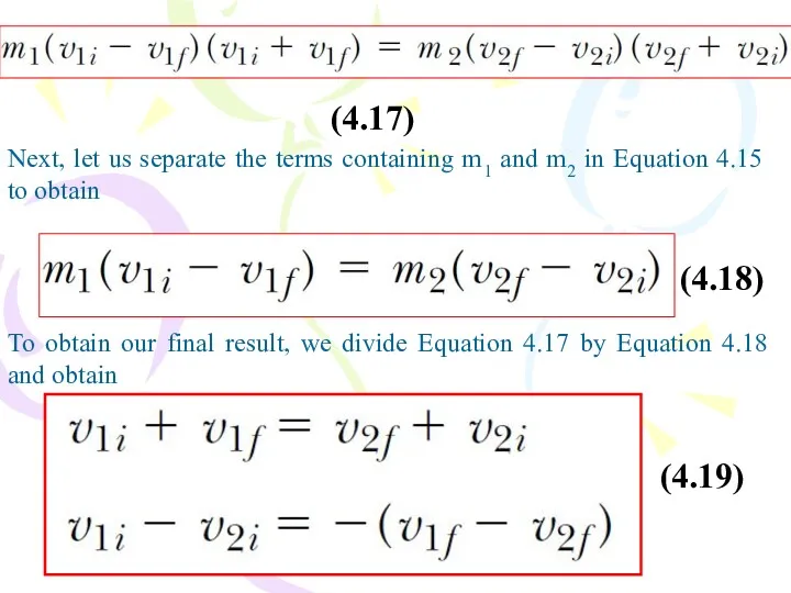
Next, let us separate the terms containing m1 and m2 in
Next, let us separate the terms containing m1 and m2 in
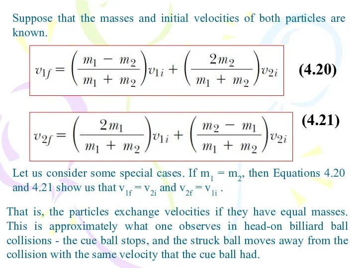
Suppose that the masses and initial velocities of both particles are
Suppose that the masses and initial velocities of both particles are
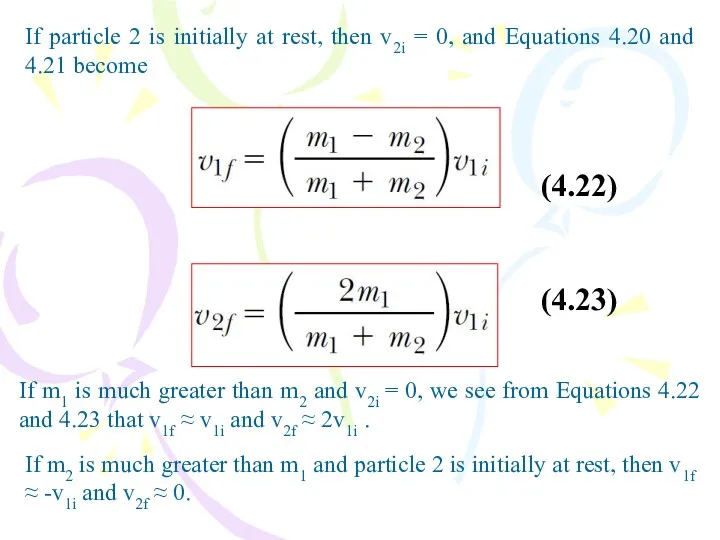
If particle 2 is initially at rest, then v2i = 0,
If particle 2 is initially at rest, then v2i = 0,
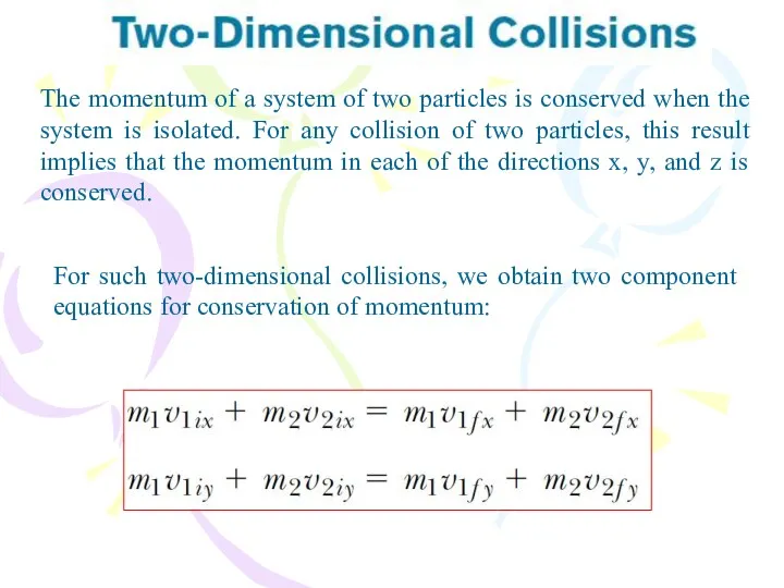
The momentum of a system of two particles is conserved when
The momentum of a system of two particles is conserved when
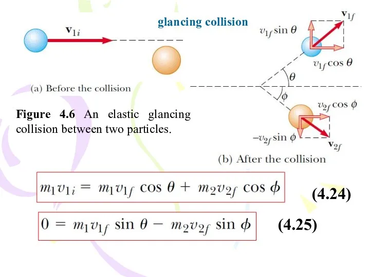
Figure 4.6 An elastic glancing collision between two particles.
glancing collision
(4.25)
(4.24)
Figure 4.6 An elastic glancing collision between two particles.
glancing collision
(4.25)
(4.24)
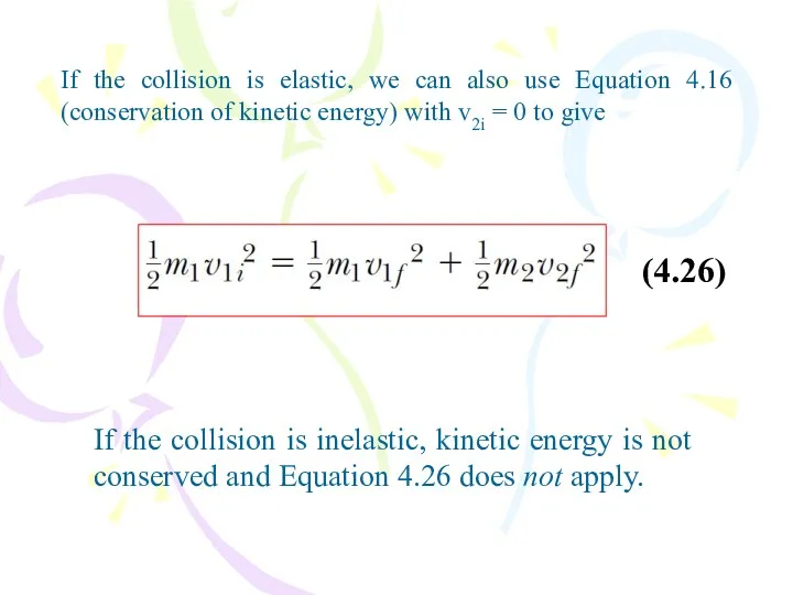
(4.26)
If the collision is elastic, we can also use Equation 4.16
(4.26)
If the collision is elastic, we can also use Equation 4.16
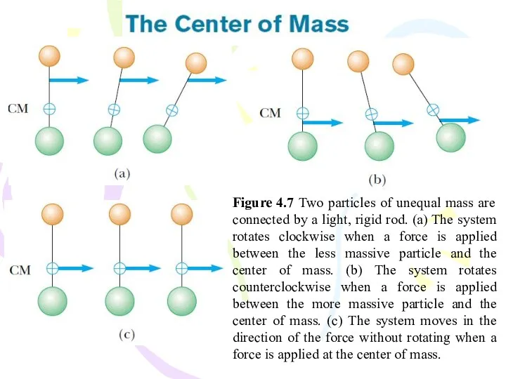
Figure 4.7 Two particles of unequal mass are connected by a
Figure 4.7 Two particles of unequal mass are connected by a
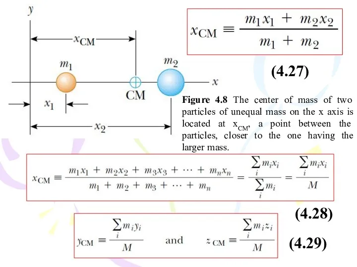
Figure 4.8 The center of mass of two particles of unequal
Figure 4.8 The center of mass of two particles of unequal
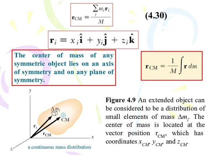
(4.30)
Figure 4.9 An extended object can be considered to be a
(4.30)
Figure 4.9 An extended object can be considered to be a
Assuming M remains constant for a system of particles, that is,
Assuming M remains constant for a system of particles, that is,
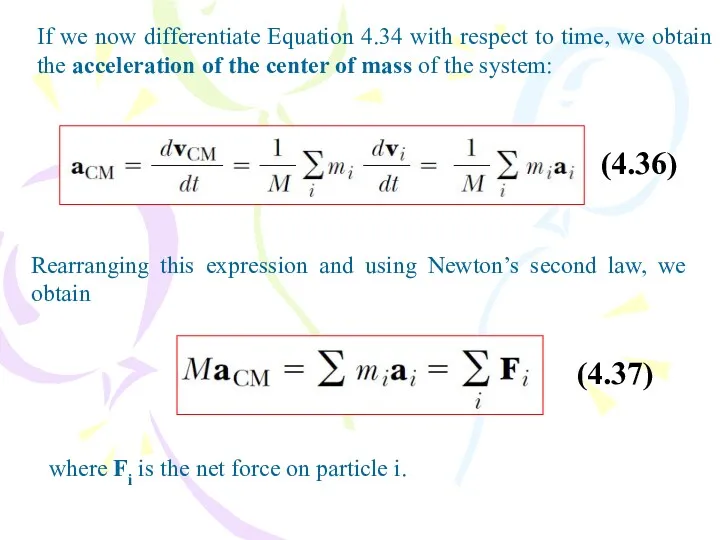
If we now differentiate Equation 4.34 with respect to time, we
If we now differentiate Equation 4.34 with respect to time, we
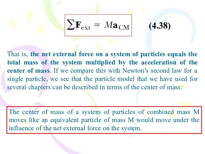
That is, the net external force on a system of particles
That is, the net external force on a system of particles
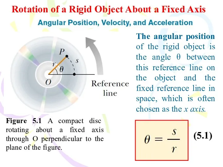
The angular position of the rigid object is the angle θ
The angular position of the rigid object is the angle θ
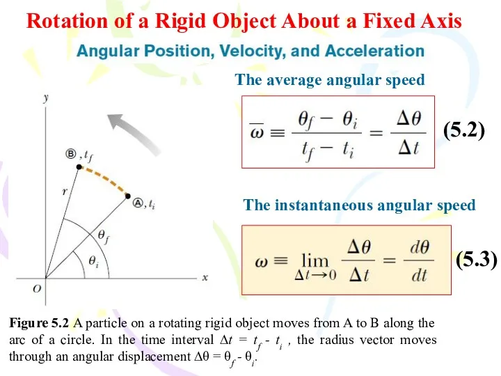
Rotation of a Rigid Object About a Fixed Axis
Figure 5.2 A
Rotation of a Rigid Object About a Fixed Axis
Figure 5.2 A
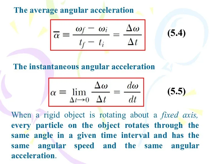
The average angular acceleration
The instantaneous angular acceleration
When a rigid object is
The average angular acceleration
The instantaneous angular acceleration
When a rigid object is
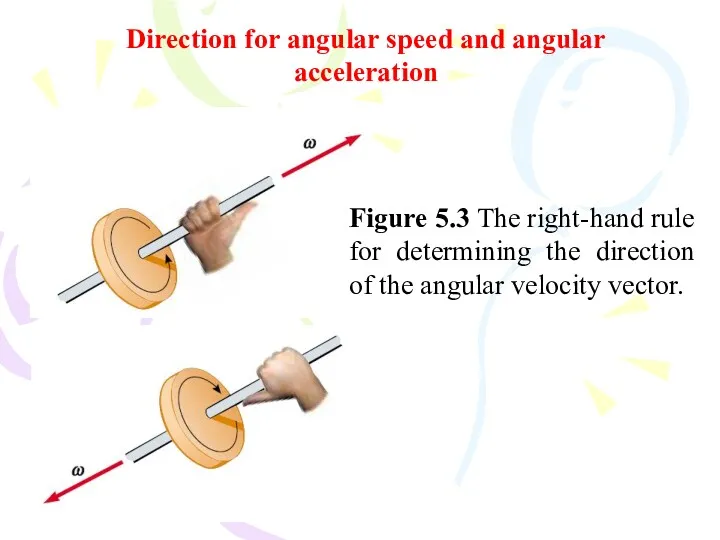
Direction for angular speed and angular acceleration
Figure 5.3 The right-hand rule
Direction for angular speed and angular acceleration
Figure 5.3 The right-hand rule
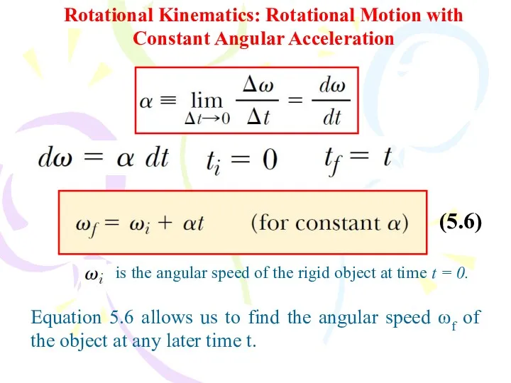
Rotational Kinematics: Rotational Motion with Constant Angular Acceleration
(5.6)
is the angular speed
Rotational Kinematics: Rotational Motion with Constant Angular Acceleration
(5.6)
is the angular speed
(5.7)
is the angular position of the rigid object at time t
(5.7)
is the angular position of the rigid object at time t
If we eliminate t from Equations 5.6 and 5.7, we obtain
This
If we eliminate t from Equations 5.6 and 5.7, we obtain
This
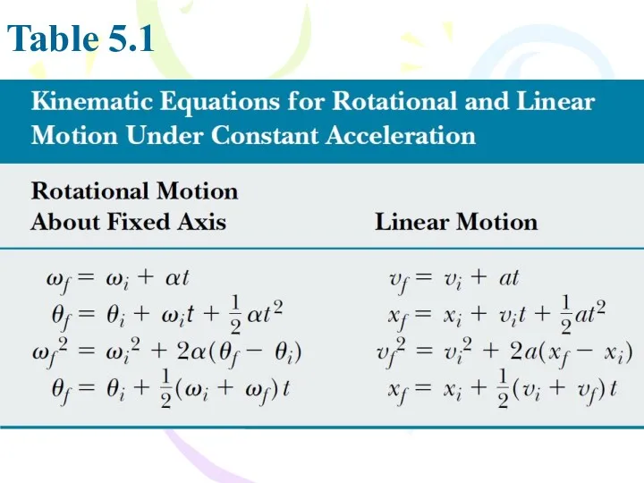
Table 5.1
Table 5.1
Angular and Linear Quantities
Figure 5.4 As a rigid object rotates about
Angular and Linear Quantities
Figure 5.4 As a rigid object rotates about
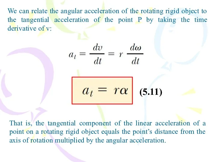
We can relate the angular acceleration of the rotating rigid object
We can relate the angular acceleration of the rotating rigid object
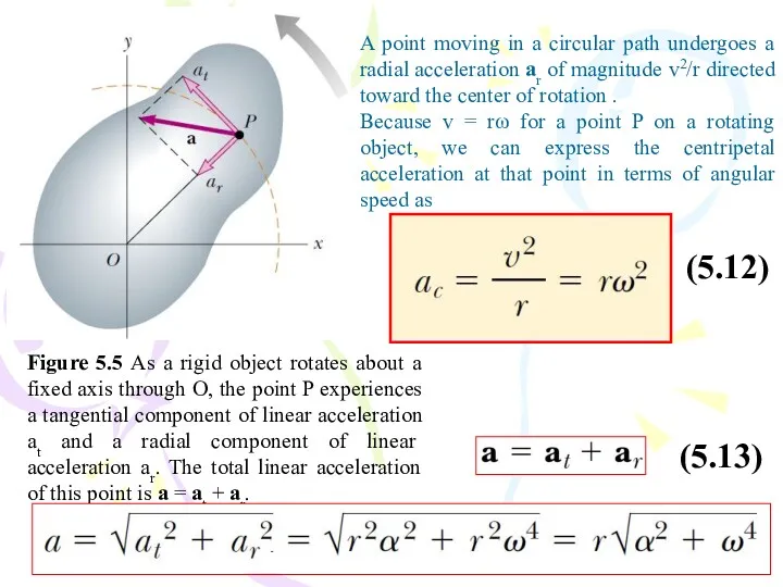
Figure 5.5 As a rigid object rotates about a fixed axis
Figure 5.5 As a rigid object rotates about a fixed axis
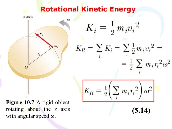
Rotational Kinetic Energy
Figure 10.7 A rigid object rotating about the z
Rotational Kinetic Energy
Figure 10.7 A rigid object rotating about the z
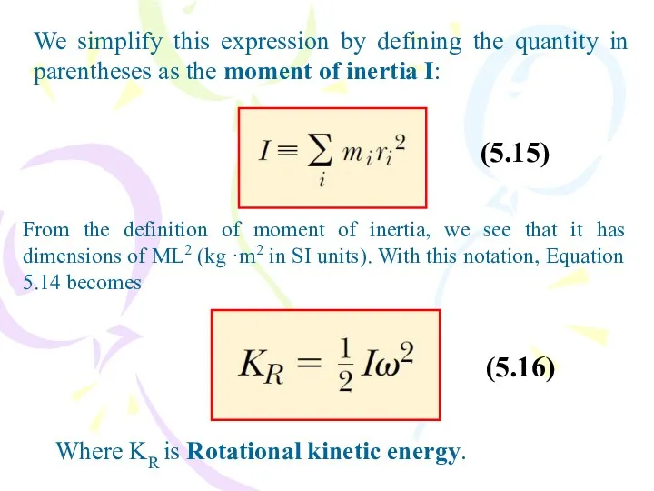
We simplify this expression by defining the quantity in parentheses as
We simplify this expression by defining the quantity in parentheses as
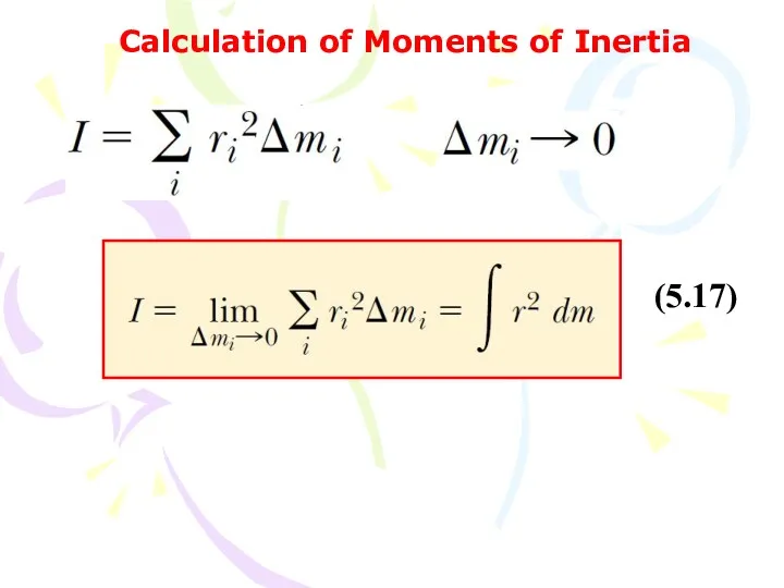
Calculation of Moments of Inertia
(5.17)
Calculation of Moments of Inertia
(5.17)
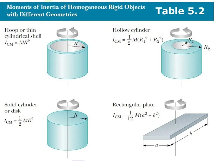
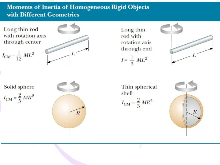
Table 5.2
Table 5.2
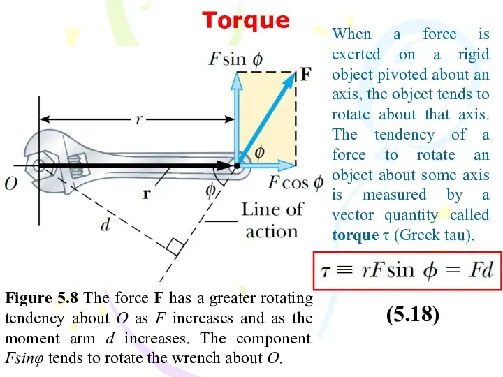
Torque
Figure 5.8 The force F has a greater rotating tendency about
Torque
Figure 5.8 The force F has a greater rotating tendency about
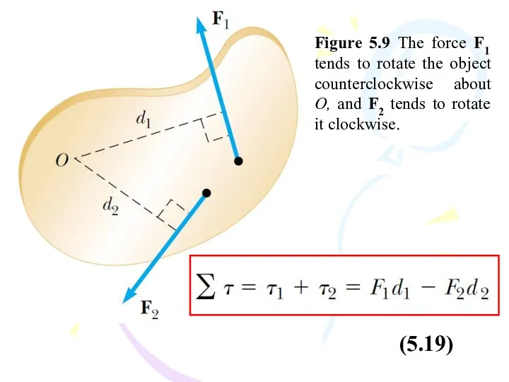
Figure 5.9 The force F1 tends to rotate the object counterclockwise
Figure 5.9 The force F1 tends to rotate the object counterclockwise
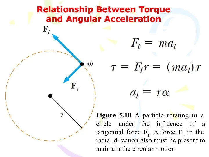
Relationship Between Torque and Angular Acceleration
Figure 5.10 A particle rotating in
Relationship Between Torque and Angular Acceleration
Figure 5.10 A particle rotating in
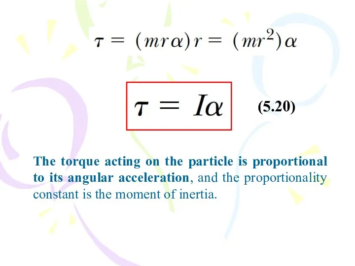
The torque acting on the particle is proportional to its angular
The torque acting on the particle is proportional to its angular
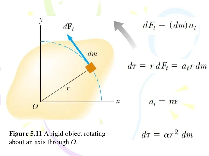
Figure 5.11 A rigid object rotating about an axis through O.
Figure 5.11 A rigid object rotating about an axis through O.
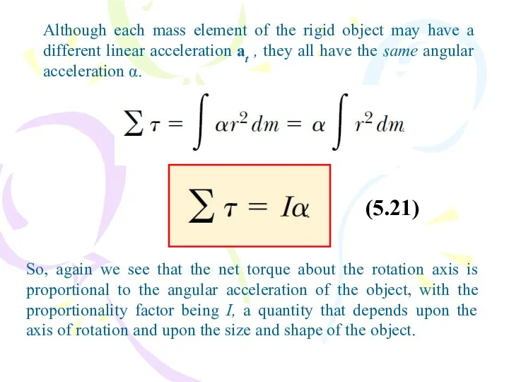
Although each mass element of the rigid object may have a
Although each mass element of the rigid object may have a
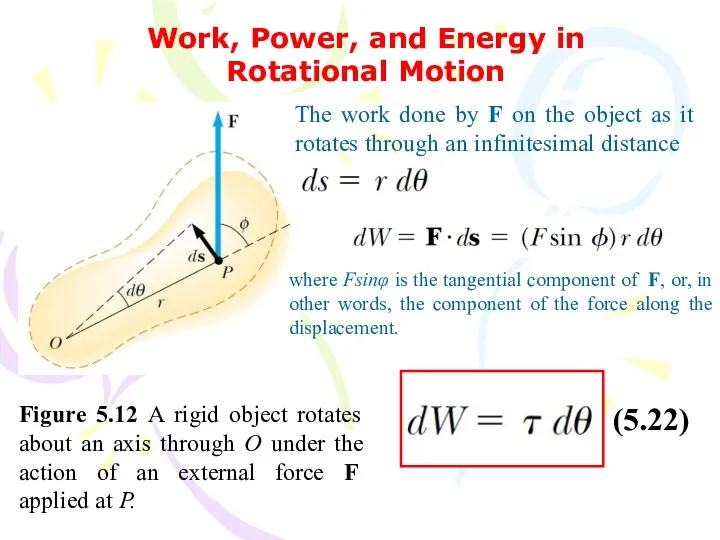
Work, Power, and Energy in Rotational Motion
Figure 5.12 A rigid object
Work, Power, and Energy in Rotational Motion
Figure 5.12 A rigid object
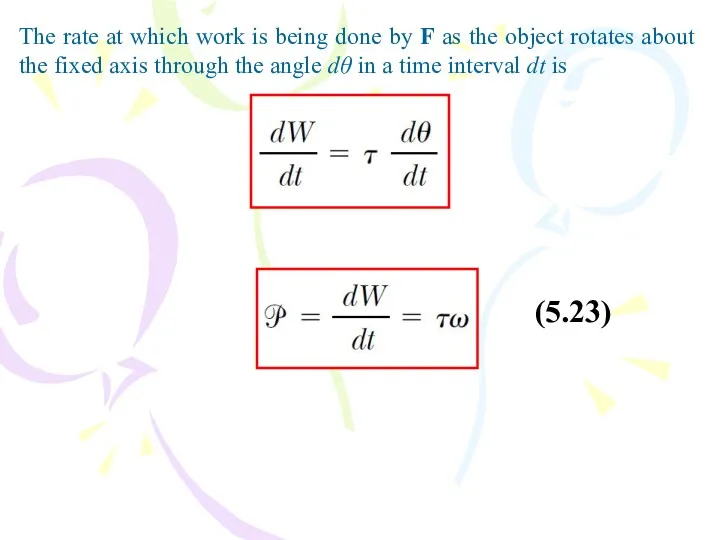
The rate at which work is being done by F as
The rate at which work is being done by F as
(5.24)
(5.24)
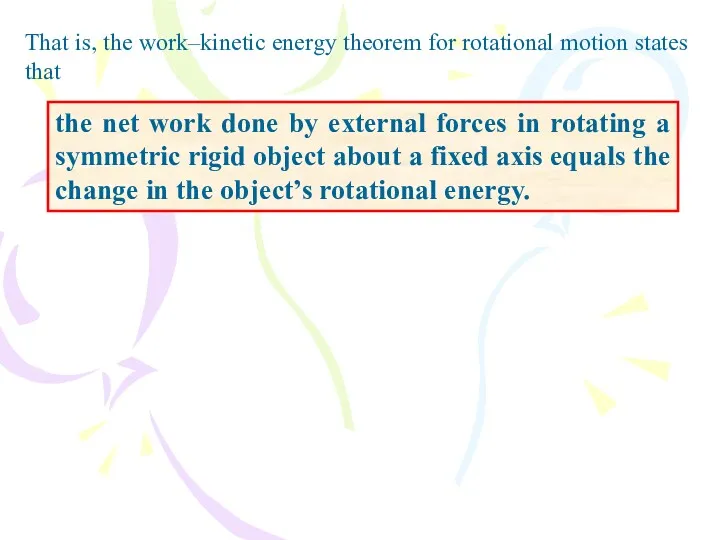
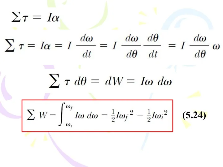
That is, the work–kinetic energy theorem for rotational motion states that
the
That is, the work–kinetic energy theorem for rotational motion states that
the
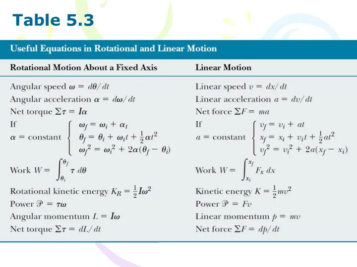
Table 5.3
Table 5.3
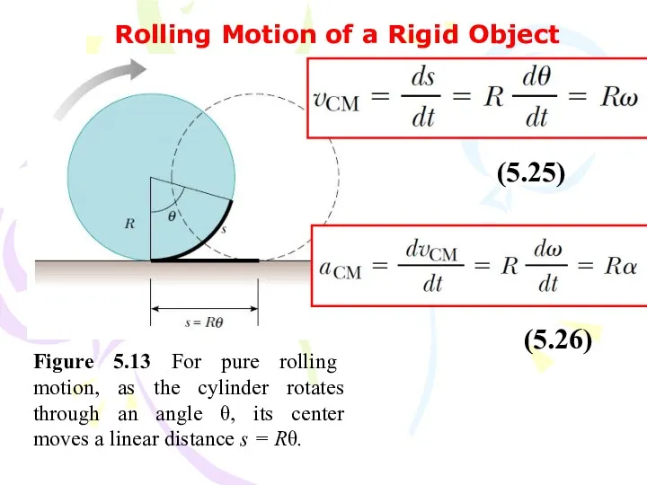
Rolling Motion of a Rigid Object
Figure 5.13 For pure rolling motion,
Rolling Motion of a Rigid Object
Figure 5.13 For pure rolling motion,
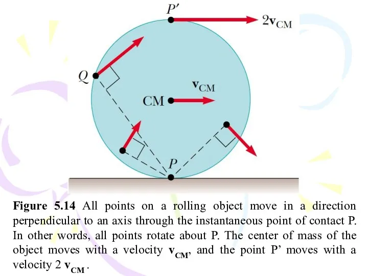
Figure 5.14 All points on a rolling object move in a
Figure 5.14 All points on a rolling object move in a
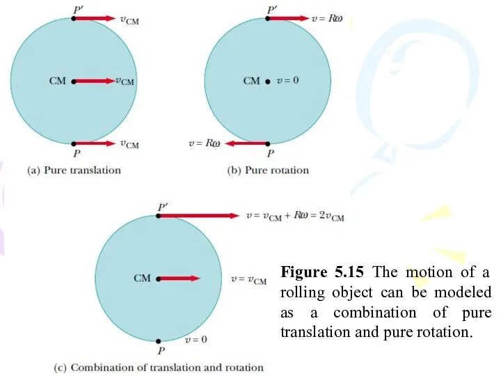
Figure 5.15 The motion of a rolling object can be modeled
Figure 5.15 The motion of a rolling object can be modeled
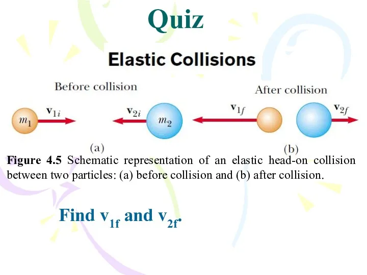
Find v1f and v2f.
Quiz
Figure 4.5 Schematic representation of an elastic
Find v1f and v2f.
Quiz
Figure 4.5 Schematic representation of an elastic
 Развитие ракетной техники
 Переменный электрический ток
 Кількість речовини. Число Авогадро. Молярна маса
 Что такое механика?
 Электрическое поле заряженных проводников. Энергия электростатического поля
 Проектировочный расчет закрытой зубчатой передачи
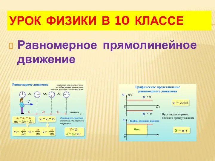 Равномерное прямолинейное движение
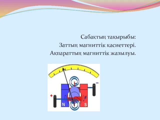 Заттың магниттік қасиеттері. Ақпараттың магниттік жазылуы
 Определение температуры (10 класс).
 Валы и оси
 Законы постоянного тока
 Зубчатые передачи
 Тема 4. Урок 17. Особенности эксплуатации оборудования для ремонта ГБЦ
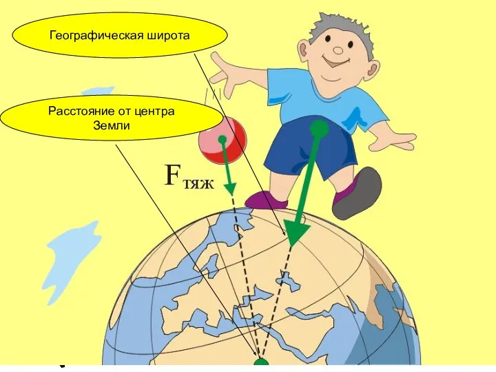 Закон всемирного тяготения
 Реактивное движение
 Электрический ток
 Электростатическое поле
 Конденсаторы, их виды и применение
 Вплив електричного поля на живі організми
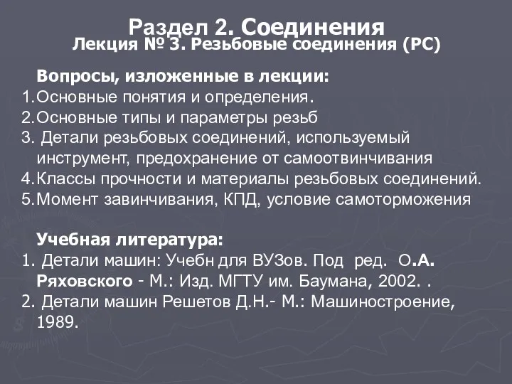 Резьбовые соединения (РС)
 Силовая передача боевой машины пехоты БМП-2. Тема 10
 Температура, способы ее измерения, температурные шкалы
 Точечные дефекты и их влияние на свойства кристаллов. Равновесные и неравновесные дефекты. Примеси в полупроводниках
 Электропроводность биологических тканей на постоянном токе
 Future cars
 Физика. Разделы физики
 Методическое сообщение по теме Повышение познавательных интересов обучающихся на основе использования информационных технологий
 Теплотехника. Второе начало термодинамики. (Лекция 5)