- Advances in Real-Time Rendering in Games

Содержание
- 2. Physically Based Lighting in Call of Duty: Black Ops Dimitar Lazarov, Lead Graphics Engineer, Treyarch
- 3. Agenda Physically based lighting and shading in the context of evolving Call of Duty’s graphics and
- 4. Performance Shapes all engine decisions and direction Built on two principles Constraints Specialization
- 5. Constrained rendering choices Forward rendering, 2x MSAA Single pass lighting All material blending inside the shader
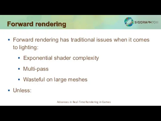
- 6. Forward rendering Forward rendering has traditional issues when it comes to lighting: Exponential shader complexity Multi-pass
- 7. Lighting constraints One primary light per surface!
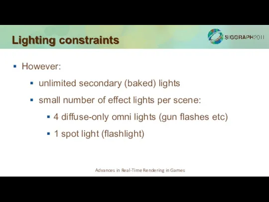
- 8. Lighting constraints However: unlimited secondary (baked) lights small number of effect lights per scene: 4 diffuse-only
- 9. Performed offline in a custom global illumination (raytracing) tool, stored in three components: Lightmaps Lightgrid Environment
- 10. Radiance vs. irradiance Irradiance (E) Radiance (L)
- 11. Run-time lighting All Primary lighting is computed in the shader A run-time shadowmap per primary overrides
- 12. Run-time lighting: diffuse Primary Diffuse Classic Lambert term Modulated by the shadow and the diffuse albedo
- 13. Run-time lighting: specular Primary Specular Microfacet BRDF Modulated by the shadow and the “diffuse” cosine factor
- 14. Why Physically-Based Crafting Physically Motivated Shading Models for Game Development (SIGGRAPH 2010): Easier to achieve photo/hyper
- 15. Why Physically-Based continued Call of Duty: Black Ops objectives: Maximize the value of the one primary
- 16. Some prerequisites Gamma correct pipeline Used gamma 2.0, mix of shader & GPU conversion HDR lighting
- 17. Microfacet theory Theory for specular reflection; assumes surface made of microfacets – tiny mirrors that reflect
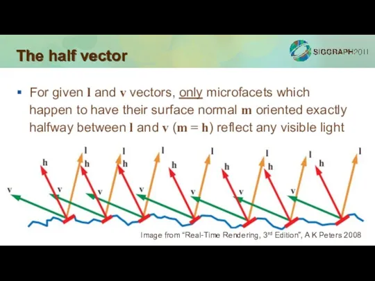
- 18. The half vector For given l and v vectors, only microfacets which happen to have their
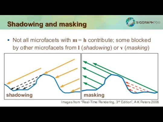
- 19. Shadowing and masking Not all microfacets with m = h contribute; some blocked by other microfacets
- 20. Microfacet BRDF
- 21. Microfacet BRDF - D
- 22. Microfacet BRDF - F
- 23. Microfacet BRDF - G
- 24. Microfacet BRDF – the rest
- 25. Modular approach Early experiments used Cook-Torrance We then tried out different options to get a more
- 26. Shading with microfacet BRDF Useful to factor into three components Distribution function times constant: Fresnel: Visibility
- 27. Distribution functions Beckmann: Read roughness m from an LDR texture (range 0 to 1)
- 28. Distribution functions continued Phong lobe NDF (Blinn-Phong): Specular power n in the range (1, 8192) Encode
- 29. Distribution functions comparison Beckmann, Phong NDFs very similar in our gloss range Blinn-Phong is cheaper to
- 30. Beckmann Distribution function
- 31. Blinn-Phong Distribution function
- 32. Distribution functions comparison m = 0.6, 0.7, 0.8, 0.9 m = 0.2, 0.3, 0.4, 0.5 Blinn-Phong
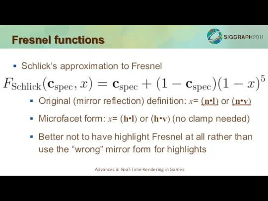
- 33. Fresnel functions Schlick’s approximation to Fresnel Original (mirror reflection) definition: x= (n•l) or (n•v) Microfacet form:
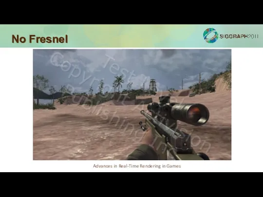
- 34. No Fresnel
- 35. Correct Fresnel
- 36. Incorrect Fresnel
- 37. Visibility functions No visibility function: Shadowing-masking function is effectively:
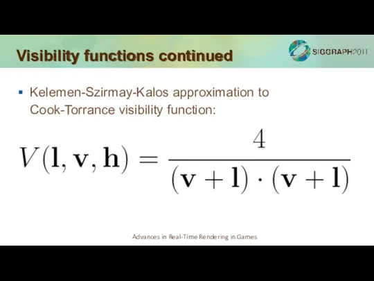
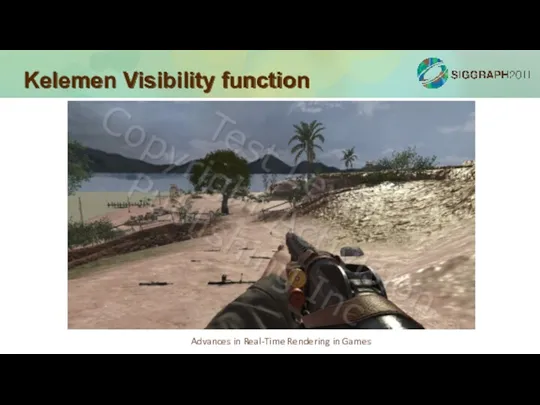
- 38. Visibility functions continued Kelemen-Szirmay-Kalos approximation to Cook-Torrance visibility function:
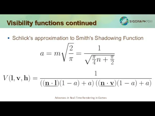
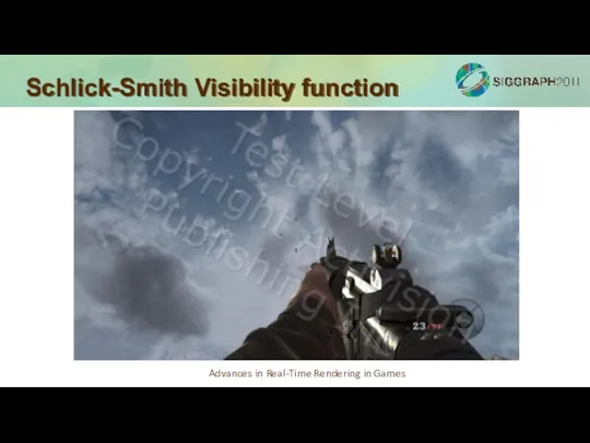
- 39. Visibility functions continued Schlick's approximation to Smith's Shadowing Function
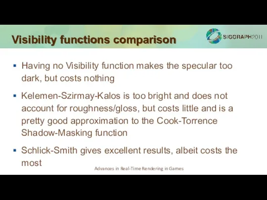
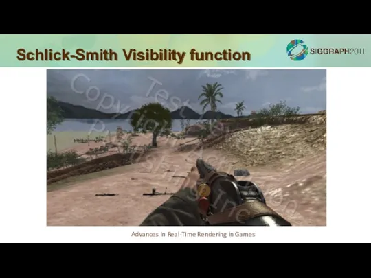
- 40. Visibility functions comparison Having no Visibility function makes the specular too dark, but costs nothing Kelemen-Szirmay-Kalos
- 41. No Visibility function
- 42. Schlick-Smith Visibility function
- 43. Kelemen Visibility function
- 44. Cook-Torrance Visibility function
- 45. Schlick-Smith Visibility function
- 46. Kelemen Visibility function
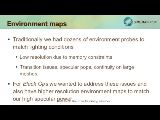
- 47. Environment maps Traditionally we had dozens of environment probes to match lighting conditions Low resolution due
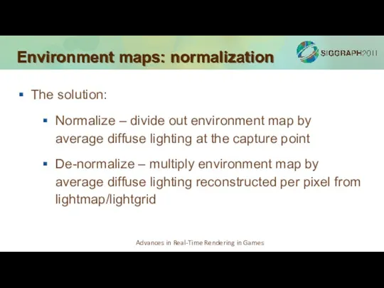
- 48. Environment maps: normalization The solution: Normalize – divide out environment map by average diffuse lighting at
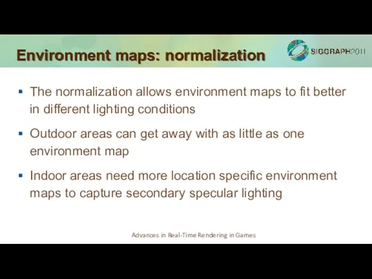
- 49. Environment maps: normalization The normalization allows environment maps to fit better in different lighting conditions Outdoor
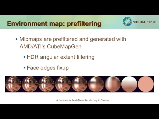
- 50. Environment map: prefiltering Mipmaps are prefiltered and generated with AMD/ATI’s CubeMapGen HDR angular extent filtering Face
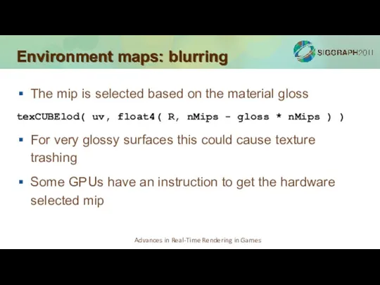
- 51. Environment maps: blurring The mip is selected based on the material gloss texCUBElod( uv, float4( R,
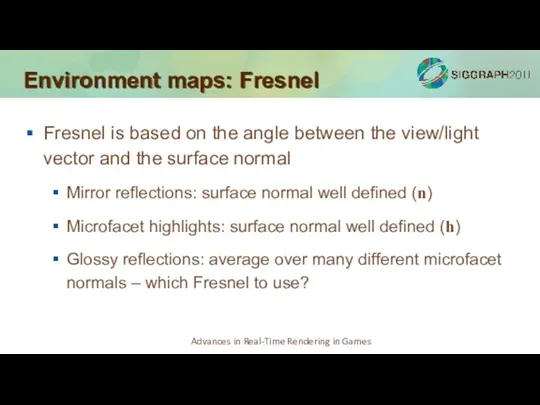
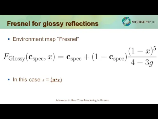
- 52. Environment maps: Fresnel Fresnel is based on the angle between the view/light vector and the surface
- 53. A full solution would involve multiple samples from the environment map and BRDF together We can’t
- 54. Fresnel for glossy reflections Environment map “Fresnel” In this case x = (n•v)
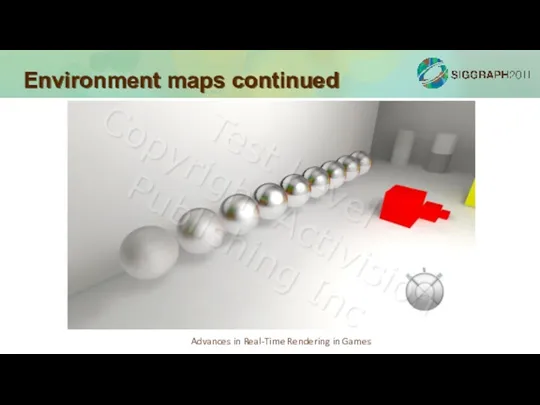
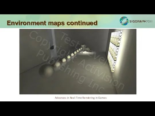
- 55. Environment maps continued
- 56. Environment maps continued
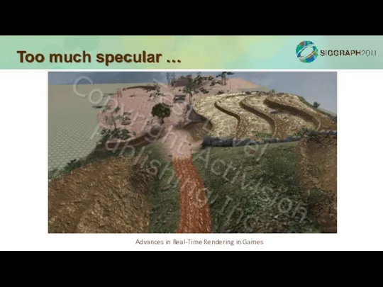
- 57. Too much specular …
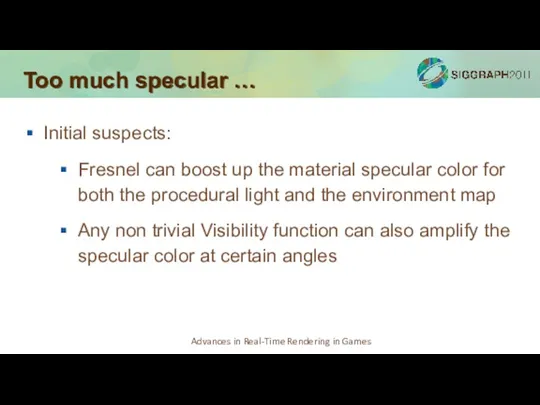
- 58. Too much specular … Initial suspects: Fresnel can boost up the material specular color for both
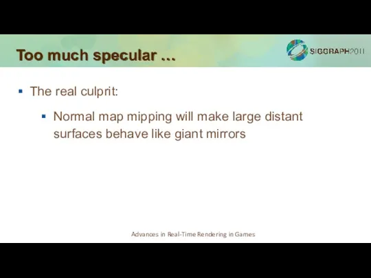
- 59. Too much specular … The real culprit: Normal map mipping will make large distant surfaces behave
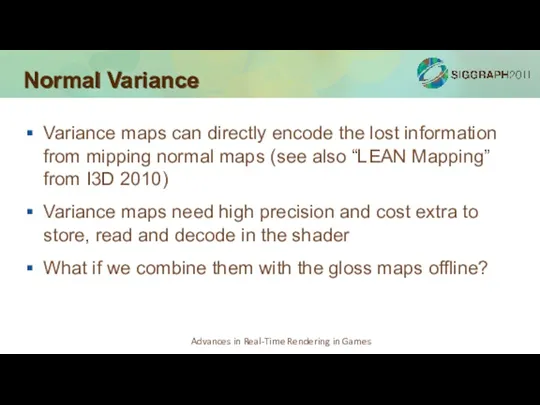
- 60. Normal Variance Variance maps can directly encode the lost information from mipping normal maps (see also
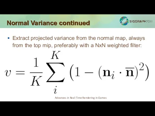
- 61. Normal Variance continued Extract projected variance from the normal map, always from the top mip, preferably
- 62. Add in the authored gloss, converted to variance: Normal Variance continued
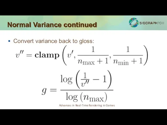
- 63. Normal Variance continued Convert variance back to gloss:
- 64. Normal Variance continued This method solved the majority of our specular intensity issues Tends to anti-alias
- 65. Without Variance-to-Gloss
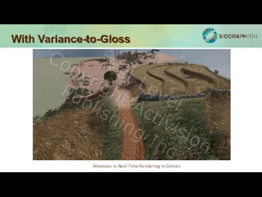
- 66. With Variance-to-Gloss
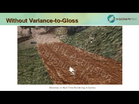
- 67. Without Variance-to-Gloss
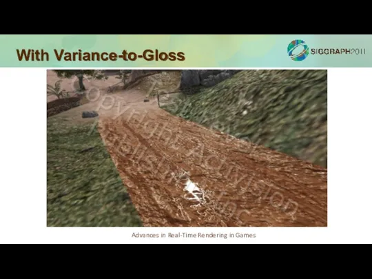
- 68. With Variance-to-Gloss
- 69. The Art perspective Even with all techniques properly implemented the “ease of authoring” still elusive Artists
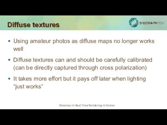
- 70. Diffuse textures Using amateur photos as diffuse maps no longer works well Diffuse textures can and
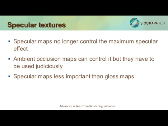
- 71. Specular textures Specular maps no longer control the maximum specular effect Ambient occlusion maps can control
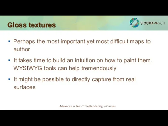
- 72. Gloss textures Perhaps the most important yet most difficult maps to author It takes time to
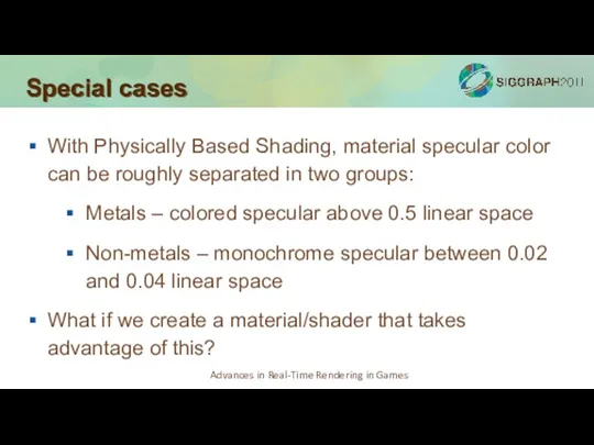
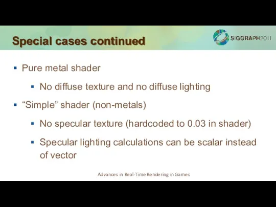
- 73. Special cases With Physically Based Shading, material specular color can be roughly separated in two groups:
- 74. Special cases continued Pure metal shader No diffuse texture and no diffuse lighting “Simple” shader (non-metals)
- 75. Performance Physically Based Shading is relatively more expensive (average 10-20% more ALU) Using special case shaders
- 76. Conclusions Physically Based Shading is totally worth it! It will make your specular truly “next gen”
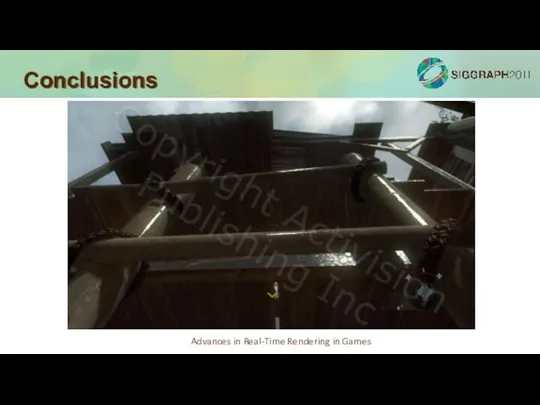
- 77. Conclusions
- 78. Thanks Natalya Tatarchuk Naty Hoffman Paul Edelstein The Call of Duty: Black Ops Team
- 79. Contact info Email me at dlazarov@treyarch.com
- 80. Bonus slides
- 81. Multiple surface bounces In reality, blocked light continues to bounce; some will eventually contribute to the
- 82. Blinn-Phong normalization Some games use (n+8) instead of (n+2) The (n+8) “Hoffman-Sloan” normalization factor first appeared
- 83. Ambient Occlusion Materials with AO maps can suppress secondary diffuse, primary and secondary specular Suppressing primary
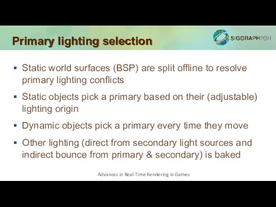
- 84. Primary lighting selection Static world surfaces (BSP) are split offline to resolve primary lighting conflicts Static
- 85. BSP
- 86. BSP + static objects
- 87. BSP + static and dynamic objects
- 88. Metalness method Two textures: color and metalness If metalness is 1 then color is treated as
- 90. Скачать презентацию
Physically Based Lighting in
Call of Duty: Black Ops
Dimitar Lazarov, Lead
Physically Based Lighting in
Call of Duty: Black Ops
Dimitar Lazarov, Lead
Agenda
Physically based lighting and shading
in the context of evolving Call of
Agenda
Physically based lighting and shading
in the context of evolving Call of
Performance
Shapes all engine decisions and direction
Built on two principles
Constraints
Specialization
Performance
Shapes all engine decisions and direction
Built on two principles
Constraints
Specialization
Constrained rendering choices
Forward rendering, 2x MSAA
Single pass lighting
All material blending inside
Constrained rendering choices
Forward rendering, 2x MSAA
Single pass lighting
All material blending inside
Forward rendering
Forward rendering has traditional issues when it comes to lighting:
Exponential
Forward rendering
Forward rendering has traditional issues when it comes to lighting:
Exponential
Lighting constraints
One primary light per surface!
Lighting constraints
One primary light per surface!
Lighting constraints
However:
unlimited secondary (baked) lights
small number of effect lights per scene:
4
Lighting constraints
However:
unlimited secondary (baked) lights
small number of effect lights per scene:
4
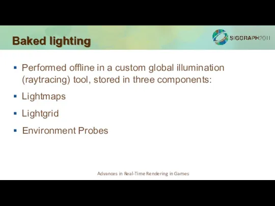
Performed offline in a custom global illumination (raytracing) tool, stored in
Performed offline in a custom global illumination (raytracing) tool, stored in
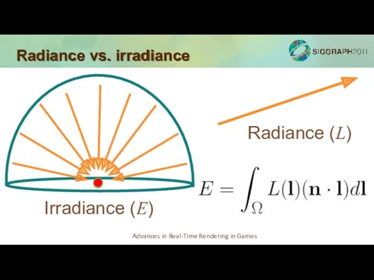
Radiance vs. irradiance
Irradiance (E)
Radiance (L)
Radiance vs. irradiance
Irradiance (E)
Radiance (L)
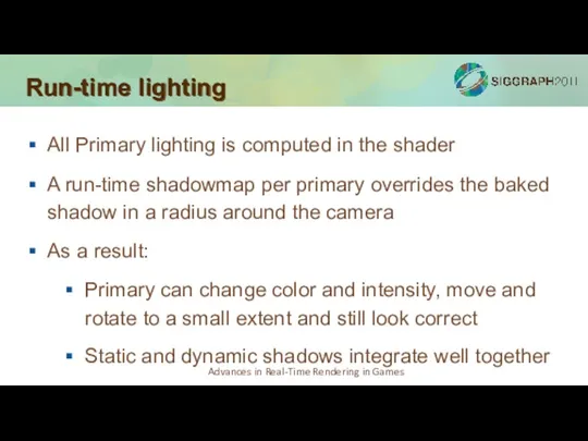
Run-time lighting
All Primary lighting is computed in the shader
A run-time shadowmap
Run-time lighting
All Primary lighting is computed in the shader
A run-time shadowmap
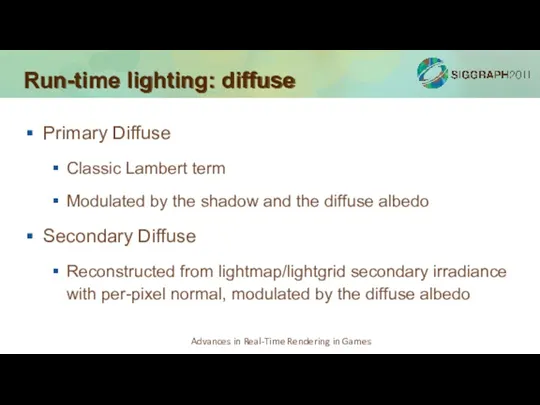
Run-time lighting: diffuse
Primary Diffuse
Classic Lambert term
Modulated by the shadow and
Run-time lighting: diffuse
Primary Diffuse
Classic Lambert term
Modulated by the shadow and
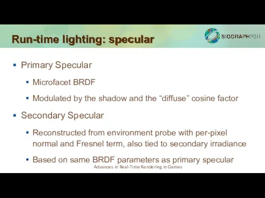
Run-time lighting: specular
Primary Specular
Microfacet BRDF
Modulated by the shadow and the “diffuse”
Run-time lighting: specular
Primary Specular
Microfacet BRDF
Modulated by the shadow and the “diffuse”
Why Physically-Based
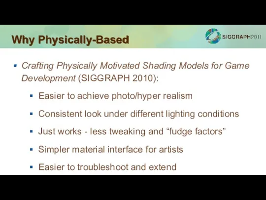
Crafting Physically Motivated Shading Models for Game Development (SIGGRAPH 2010):
Easier
Why Physically-Based
Crafting Physically Motivated Shading Models for Game Development (SIGGRAPH 2010):
Easier
Why Physically-Based continued
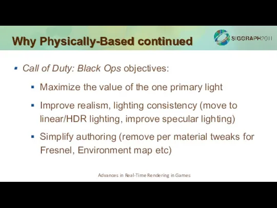
Call of Duty: Black Ops objectives:
Maximize the value of
Why Physically-Based continued
Call of Duty: Black Ops objectives:
Maximize the value of
Some prerequisites
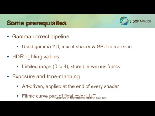
Gamma correct pipeline
Used gamma 2.0, mix of shader & GPU
Some prerequisites
Gamma correct pipeline
Used gamma 2.0, mix of shader & GPU
Microfacet theory
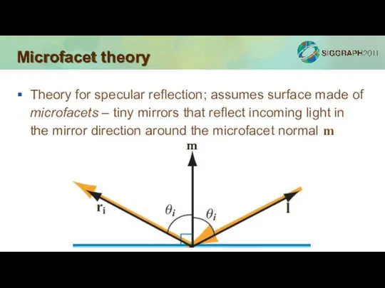
Theory for specular reflection; assumes surface made of microfacets –
Microfacet theory
Theory for specular reflection; assumes surface made of microfacets –
The half vector
For given l and v vectors, only microfacets which
The half vector
For given l and v vectors, only microfacets which
Shadowing and masking
Not all microfacets with m = h contribute; some
Shadowing and masking
Not all microfacets with m = h contribute; some
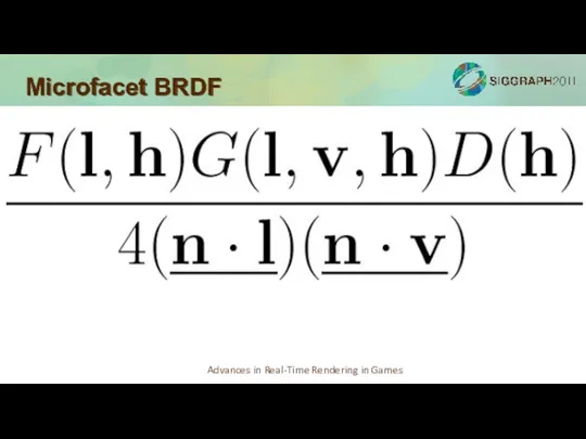
Microfacet BRDF
Microfacet BRDF
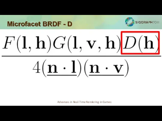
Microfacet BRDF - D
Microfacet BRDF - D
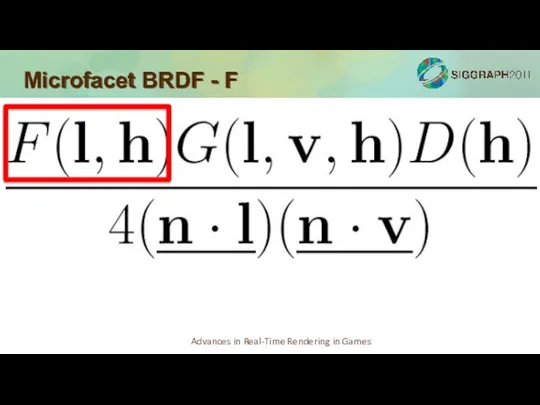
Microfacet BRDF - F
Microfacet BRDF - F
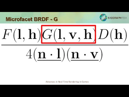
Microfacet BRDF - G
Microfacet BRDF - G
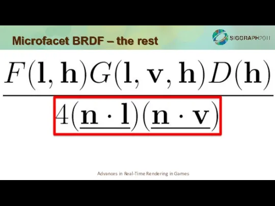
Microfacet BRDF – the rest
Microfacet BRDF – the rest
Modular approach
Early experiments used Cook-Torrance
We then tried out different options to
Modular approach
Early experiments used Cook-Torrance
We then tried out different options to
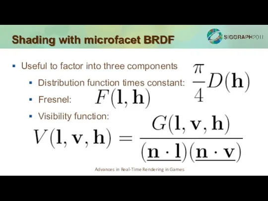
Shading with microfacet BRDF
Useful to factor into three components
Distribution function times
Shading with microfacet BRDF
Useful to factor into three components
Distribution function times
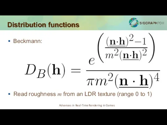
Distribution functions
Beckmann:
Read roughness m from an LDR texture (range 0 to
Distribution functions
Beckmann:
Read roughness m from an LDR texture (range 0 to
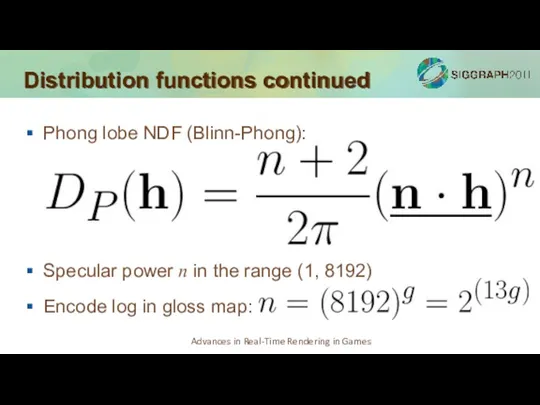
Distribution functions continued
Phong lobe NDF (Blinn-Phong):
Specular power n in the range
Distribution functions continued
Phong lobe NDF (Blinn-Phong):
Specular power n in the range
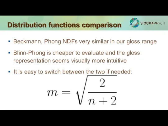
Distribution functions comparison
Beckmann, Phong NDFs very similar in our gloss range
Blinn-Phong
Distribution functions comparison
Beckmann, Phong NDFs very similar in our gloss range
Blinn-Phong
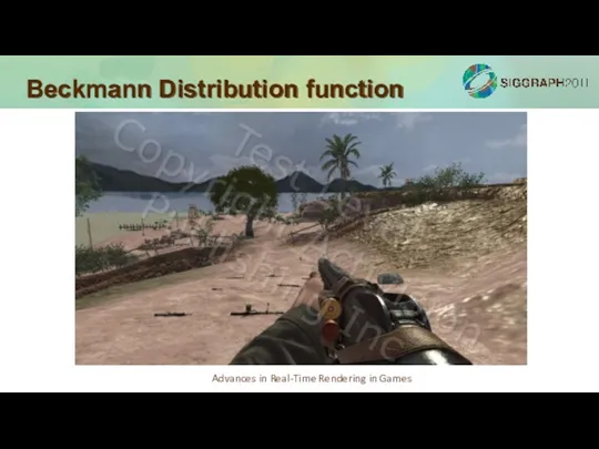
Beckmann Distribution function
Beckmann Distribution function
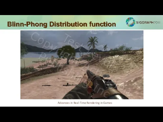
Blinn-Phong Distribution function
Blinn-Phong Distribution function
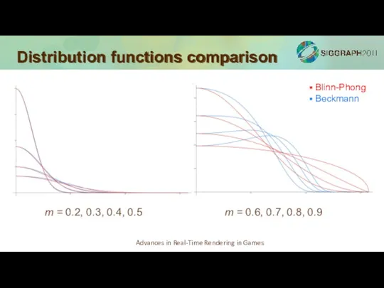
Distribution functions comparison
m = 0.6, 0.7, 0.8, 0.9
m = 0.2, 0.3, 0.4, 0.5
Distribution functions comparison
m = 0.6, 0.7, 0.8, 0.9
m = 0.2, 0.3, 0.4, 0.5
Fresnel functions
Schlick’s approximation to Fresnel
Original (mirror reflection) definition: x= (n•l) or
Fresnel functions
Schlick’s approximation to Fresnel
Original (mirror reflection) definition: x= (n•l) or
No Fresnel
No Fresnel
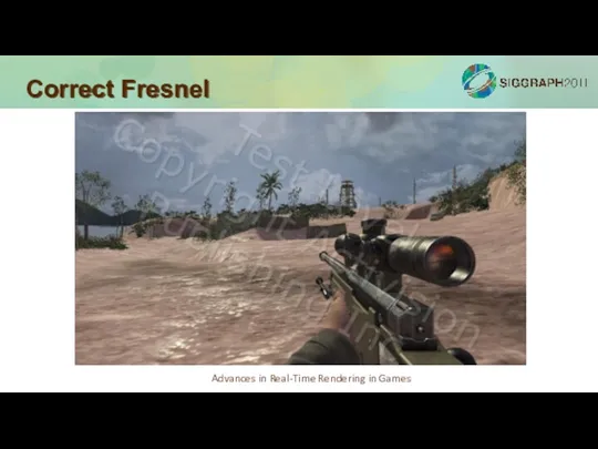
Correct Fresnel
Correct Fresnel
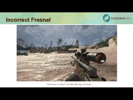
Incorrect Fresnel
Incorrect Fresnel
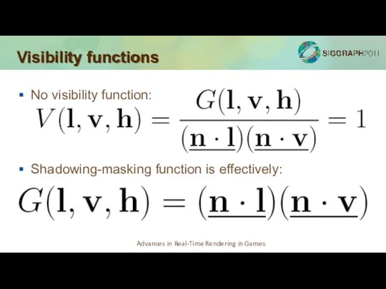
Visibility functions
No visibility function:
Shadowing-masking function is effectively:
Visibility functions
No visibility function:
Shadowing-masking function is effectively:
Visibility functions continued
Kelemen-Szirmay-Kalos approximation to Cook-Torrance visibility function:
Visibility functions continued
Kelemen-Szirmay-Kalos approximation to Cook-Torrance visibility function:
Visibility functions continued
Schlick's approximation to Smith's Shadowing Function
Visibility functions continued
Schlick's approximation to Smith's Shadowing Function
Visibility functions comparison
Having no Visibility function makes the specular too dark,
Visibility functions comparison
Having no Visibility function makes the specular too dark,
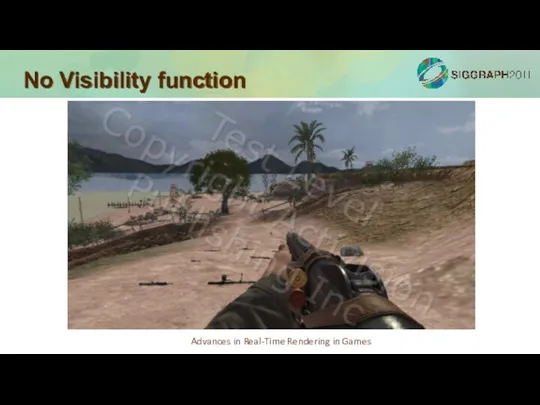
No Visibility function
No Visibility function
Schlick-Smith Visibility function
Schlick-Smith Visibility function
Kelemen Visibility function
Kelemen Visibility function
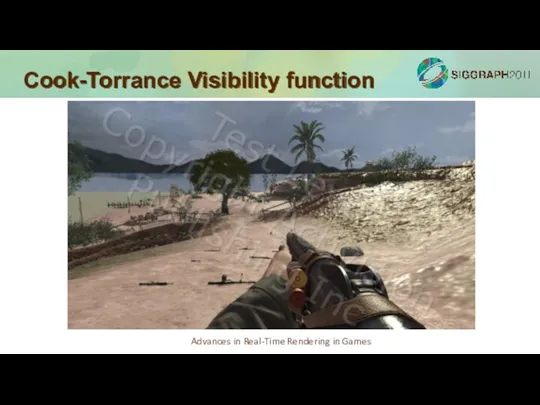
Cook-Torrance Visibility function
Cook-Torrance Visibility function
Schlick-Smith Visibility function
Schlick-Smith Visibility function
Kelemen Visibility function
Kelemen Visibility function
Environment maps
Traditionally we had dozens of environment probes to match lighting
Environment maps
Traditionally we had dozens of environment probes to match lighting
Environment maps: normalization
The solution:
Normalize – divide out environment map by average
Environment maps: normalization
The solution:
Normalize – divide out environment map by average
Environment maps: normalization
The normalization allows environment maps to fit better in
Environment maps: normalization
The normalization allows environment maps to fit better in
Environment map: prefiltering
Mipmaps are prefiltered and generated with AMD/ATI’s CubeMapGen
HDR angular
Environment map: prefiltering
Mipmaps are prefiltered and generated with AMD/ATI’s CubeMapGen
HDR angular
Environment maps: blurring
The mip is selected based on the material gloss
Environment maps: blurring
The mip is selected based on the material gloss
Environment maps: Fresnel
Fresnel is based on the angle between the view/light
Environment maps: Fresnel
Fresnel is based on the angle between the view/light
A full solution would involve multiple samples from the environment map
A full solution would involve multiple samples from the environment map
Fresnel for glossy reflections
Environment map “Fresnel”
In this case x = (n•v)
Fresnel for glossy reflections
Environment map “Fresnel”
In this case x = (n•v)
Environment maps continued
Environment maps continued
Environment maps continued
Environment maps continued
Too much specular …
Too much specular …
Too much specular …
Initial suspects:
Fresnel can boost up the material specular
Too much specular …
Initial suspects:
Fresnel can boost up the material specular
Too much specular …
The real culprit:
Normal map mipping will make large
Too much specular …
The real culprit:
Normal map mipping will make large
Normal Variance
Variance maps can directly encode the lost information from mipping
Normal Variance
Variance maps can directly encode the lost information from mipping
Normal Variance continued
Extract projected variance from the normal map, always from
Normal Variance continued
Extract projected variance from the normal map, always from
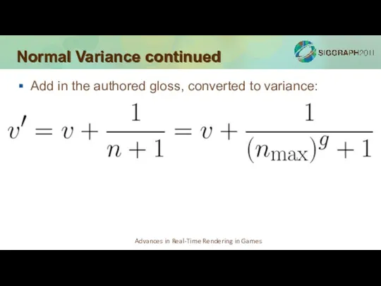
Add in the authored gloss, converted to variance:
Normal Variance continued
Add in the authored gloss, converted to variance:
Normal Variance continued
Normal Variance continued
Convert variance back to gloss:
Normal Variance continued
Convert variance back to gloss:
Normal Variance continued
This method solved the majority of our specular intensity
Normal Variance continued
This method solved the majority of our specular intensity
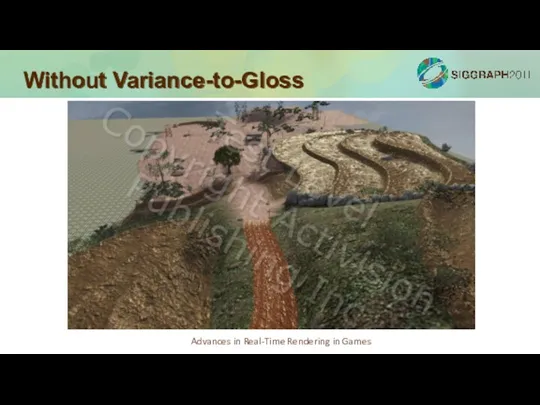
Without Variance-to-Gloss
Without Variance-to-Gloss
With Variance-to-Gloss
With Variance-to-Gloss
Without Variance-to-Gloss
Without Variance-to-Gloss
With Variance-to-Gloss
With Variance-to-Gloss
The Art perspective
Even with all techniques properly implemented the “ease of
The Art perspective
Even with all techniques properly implemented the “ease of
Diffuse textures
Using amateur photos as diffuse maps no longer works well
Diffuse
Diffuse textures
Using amateur photos as diffuse maps no longer works well
Diffuse
Specular textures
Specular maps no longer control the maximum specular effect
Ambient occlusion
Specular textures
Specular maps no longer control the maximum specular effect
Ambient occlusion
Gloss textures
Perhaps the most important yet most difficult maps to author
It
Gloss textures
Perhaps the most important yet most difficult maps to author
It
Special cases
With Physically Based Shading, material specular color can be roughly
Special cases
With Physically Based Shading, material specular color can be roughly
Special cases continued
Pure metal shader
No diffuse texture and no diffuse lighting
“Simple”
Special cases continued
Pure metal shader
No diffuse texture and no diffuse lighting
“Simple”
Performance
Physically Based Shading is relatively more expensive (average 10-20% more ALU)
Using
Performance
Physically Based Shading is relatively more expensive (average 10-20% more ALU)
Using
Conclusions
Physically Based Shading is totally worth it! It will make your
Conclusions
Physically Based Shading is totally worth it! It will make your
Conclusions
Conclusions
Thanks
Natalya Tatarchuk
Naty Hoffman
Paul Edelstein
The Call of Duty: Black Ops Team
Thanks
Natalya Tatarchuk
Naty Hoffman
Paul Edelstein
The Call of Duty: Black Ops Team

Contact info
Email me at dlazarov@treyarch.com
Contact info
Email me at dlazarov@treyarch.com

Bonus slides
Bonus slides
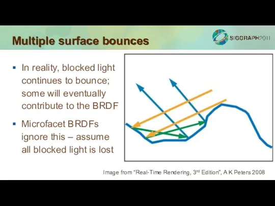
Multiple surface bounces
In reality, blocked light continues to bounce; some will
Multiple surface bounces
In reality, blocked light continues to bounce; some will
Blinn-Phong normalization
Some games use (n+8) instead of (n+2)
The (n+8) “Hoffman-Sloan” normalization
Blinn-Phong normalization
Some games use (n+8) instead of (n+2)
The (n+8) “Hoffman-Sloan” normalization
Ambient Occlusion
Materials with AO maps can suppress secondary diffuse, primary and
Ambient Occlusion
Materials with AO maps can suppress secondary diffuse, primary and
Primary lighting selection
Static world surfaces (BSP) are split offline to resolve
Primary lighting selection
Static world surfaces (BSP) are split offline to resolve
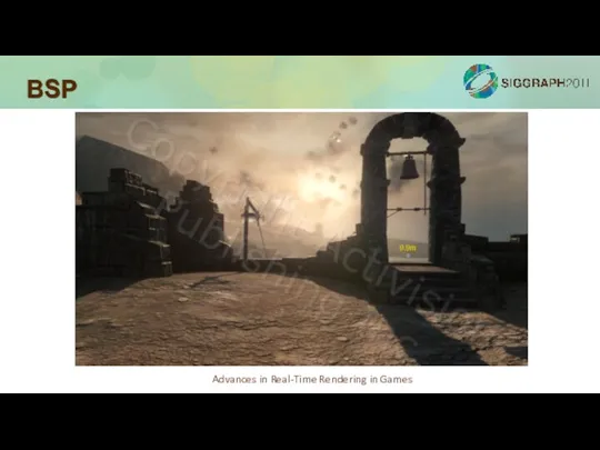
BSP
BSP
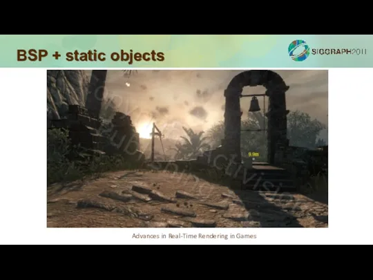
BSP + static objects
BSP + static objects
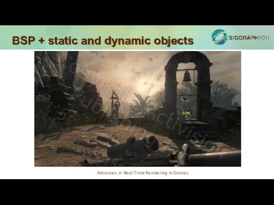
BSP + static and dynamic objects
BSP + static and dynamic objects
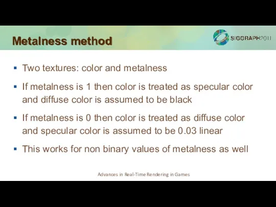
Metalness method
Two textures: color and metalness
If metalness is 1 then color
Metalness method
Two textures: color and metalness
If metalness is 1 then color
 Алгоритм. Способы записи алгоритмов
 Архитектура ЭВМ. Операционные системы. Файл
 Профессиональные информационные ресурсы. Типы литературы и виды документов. (Тема 2)
 Система AutoCAD. Общая характеристика и функциональные возможности. (Лекция 5)
 Ғылыми зерттеулердегі ақпараттық технологиялар
 Эталонная модель взаимодействия открытых систем. Основы сетевых технологий. Лекция 2
 Gretel updating software
 Разработка веб-приложения личного календаря
 Программирование на языке C#
 Формализация моделей
 Оператор цикла While. ОТП, 6 класс, урок 2
 Разветвляющиеся алгоритмы
 Киберспорт e-Sports
 Презентация, задание к уроку, домашнее задание к уроку информатики в 5 классе по теме Основная позиция пальцев на клавиатуре
 Файловые системы операционных систем MS DOS и Windows
 Работа с данными в Entity Framework Core. Проектирование и разработка веб-сервисов
 Информация и знания
 Информационный потенциал общества. (Лекция 2)
 1С Документооборот.КОРП (1)
 Електронне спілкування
 Условный оператор
 Экономическая информация (по функции управления)
 Uvers - A New Generation Social Network
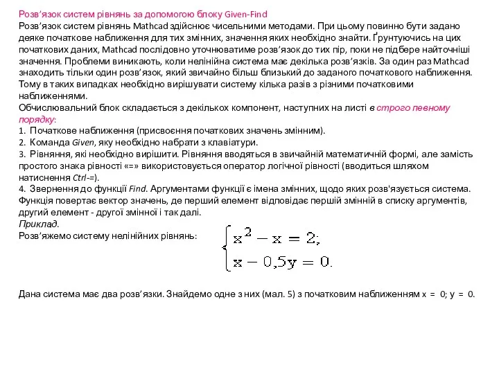 Розв’язок систем рівнянь за допомогою блоку Given-Find, Mathcad
 Использование информационных технологий на уроке математики
 Agile Engineering Services you can rely
 Представление и кодирование информации
 The Python Programming Language