- Business Statistics

Содержание
- 2. About Applied Statistics
- 4. Data Structures Classifying the Various Types of Data Sets Data can come to you in several
- 5. Univariate Data Univariate (one-variable) data sets have just one piece of information recorded for each item.
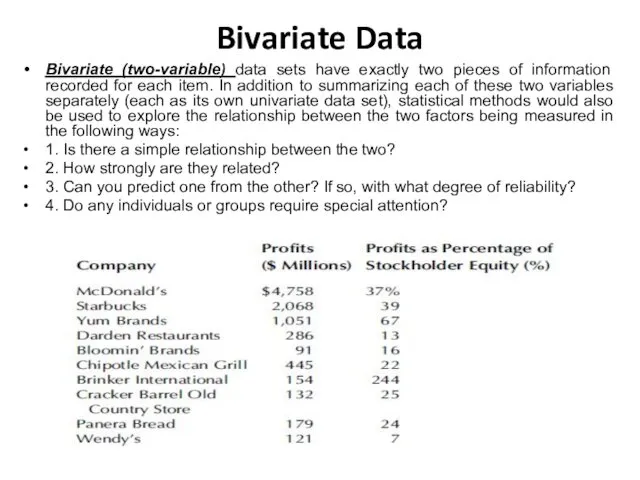
- 6. Bivariate Data Bivariate (two-variable) data sets have exactly two pieces of information recorded for each item.
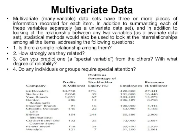
- 7. Multivariate Data Multivariate (many-variable) data sets have three or more pieces of information recorded for each
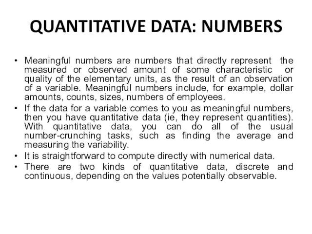
- 9. QUANTITATIVE DATA: NUMBERS Meaningful numbers are numbers that directly represent the measured or observed amount of
- 10. Discrete data is a count that can't be made more precise. Typically it involves integers. For
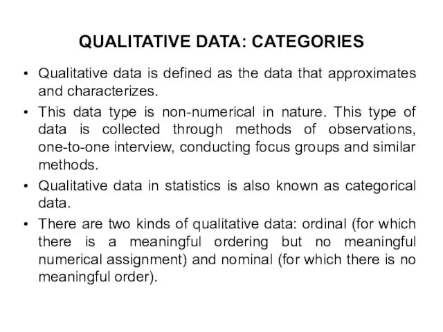
- 11. QUALITATIVE DATA: CATEGORIES Qualitative data is defined as the data that approximates and characterizes. This data
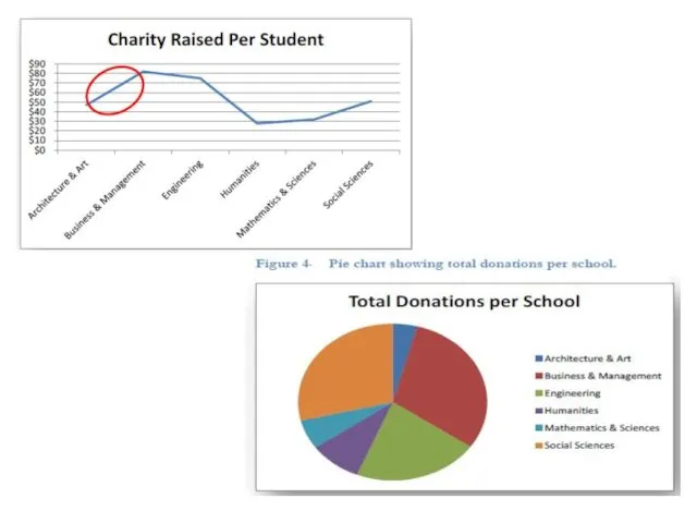
- 12. Charts, Histograms, Graphing
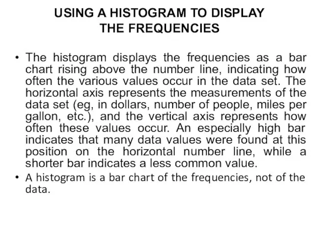
- 14. USING A HISTOGRAM TO DISPLAY THE FREQUENCIES The histogram displays the frequencies as a bar chart
- 15. Creating Frequency Distributions and Histograms in EXCEL
- 16. Consider the interest rate for 25-year fixed-rate home mortgages charged by mortgage companies in Seattle
- 20. NORMAL DISTRIBUTIONS A normal distribution is an idealized, smooth, bell-shaped histogram with all of the randomness
- 22. There are actually many different normal distributions, all symmetrically bell-shaped. They differ in that the center
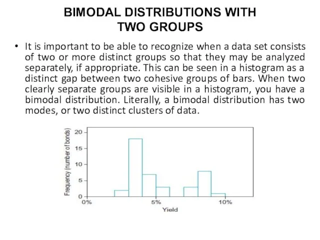
- 24. BIMODAL DISTRIBUTIONS WITH TWO GROUPS It is important to be able to recognize when a data
- 25. Task 1. Using the table below build different types of charts and graphing
- 26. TASK 2 Consider the yields (as an interest rate, in percent per year) of municipal bonds,
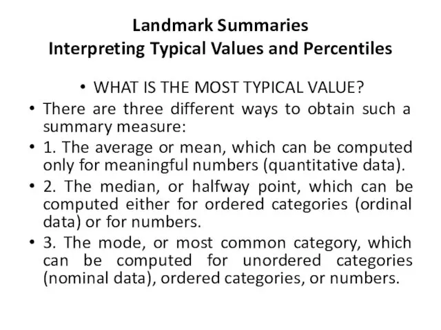
- 27. Landmark Summaries Interpreting Typical Values and Percentiles WHAT IS THE MOST TYPICAL VALUE? There are three
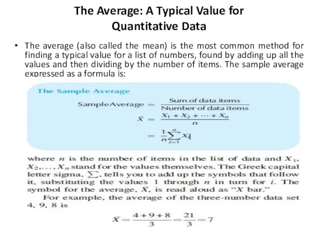
- 28. The Average: A Typical Value for Quantitative Data The average (also called the mean) is the
- 30. Excel’s Average function
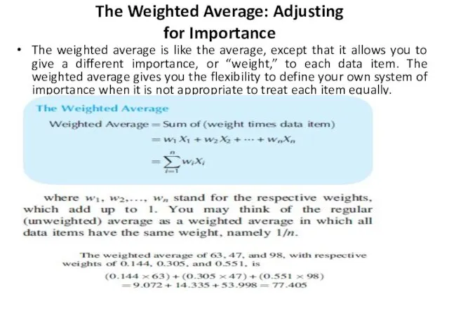
- 33. The Weighted Average: Adjusting for Importance The weighted average is like the average, except that it
- 35. The Median: A Typical Value for Quantitative and Ordinal Data The median is the middle value;
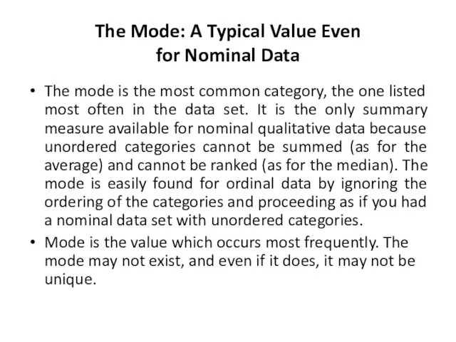
- 38. The Mode: A Typical Value Even for Nominal Data The mode is the most common category,
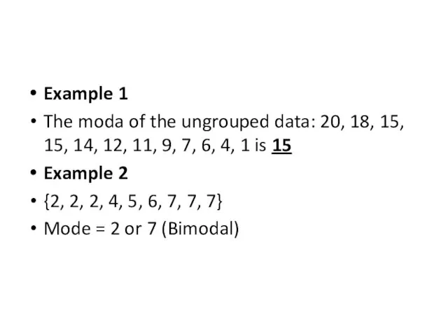
- 39. Example 1 The moda of the ungrouped data: 20, 18, 15, 15, 14, 12, 11, 9,
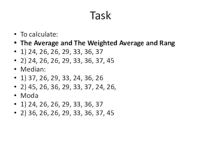
- 41. Task To calculate: The Average and The Weighted Average and Rang 1) 24, 26, 26, 29,
- 42. Consider the profits of health care companies in the Fortune 500, as shown in Table 4.3.3
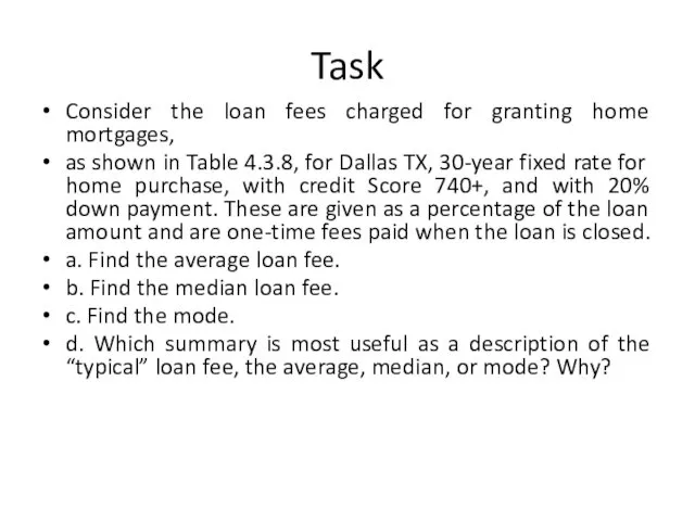
- 43. Task Consider the loan fees charged for granting home mortgages, as shown in Table 4.3.8, for
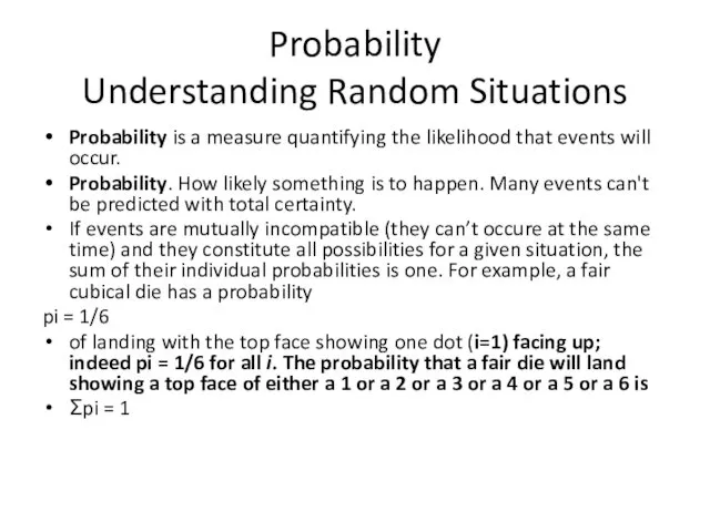
- 45. Probability Understanding Random Situations Probability is a measure quantifying the likelihood that events will occur. Probability.
- 46. A probability tree is a picture indicating probabilities and conditional probabilities for combinations of two or
- 48. Скачать презентацию
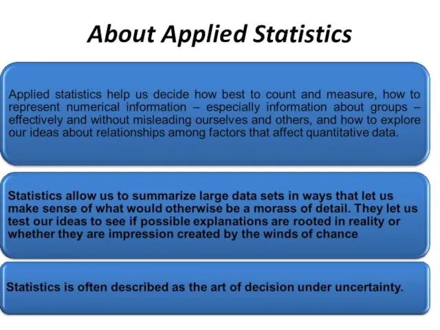
About Applied Statistics
About Applied Statistics
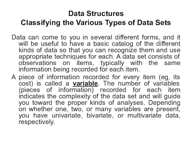
Data Structures
Classifying the Various Types of Data Sets
Data can come to
Data Structures
Classifying the Various Types of Data Sets
Data can come to
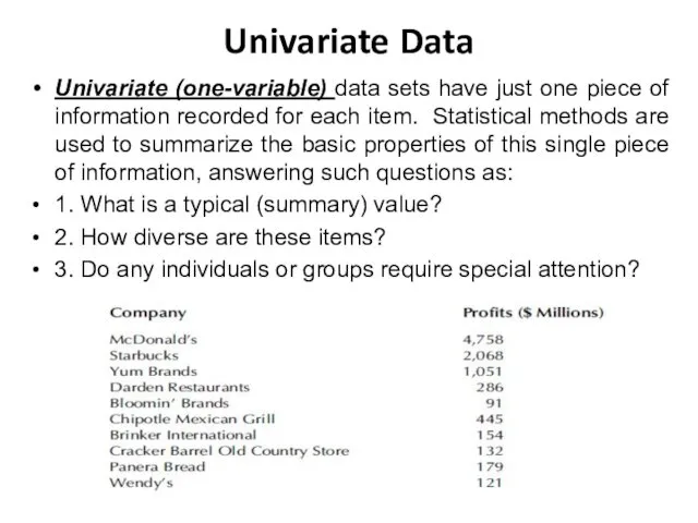
Univariate Data
Univariate (one-variable) data sets have just one piece of information
Univariate Data
Univariate (one-variable) data sets have just one piece of information
Bivariate Data
Bivariate (two-variable) data sets have exactly two pieces of information
Bivariate Data
Bivariate (two-variable) data sets have exactly two pieces of information
Multivariate Data
Multivariate (many-variable) data sets have three or more pieces of
Multivariate Data
Multivariate (many-variable) data sets have three or more pieces of

QUANTITATIVE DATA: NUMBERS
Meaningful numbers are numbers that directly represent the measured
QUANTITATIVE DATA: NUMBERS
Meaningful numbers are numbers that directly represent the measured
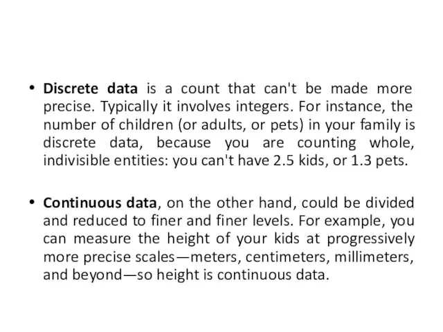
Discrete data is a count that can't be made more precise.
Discrete data is a count that can't be made more precise.
QUALITATIVE DATA: CATEGORIES
Qualitative data is defined as the data that approximates
QUALITATIVE DATA: CATEGORIES
Qualitative data is defined as the data that approximates
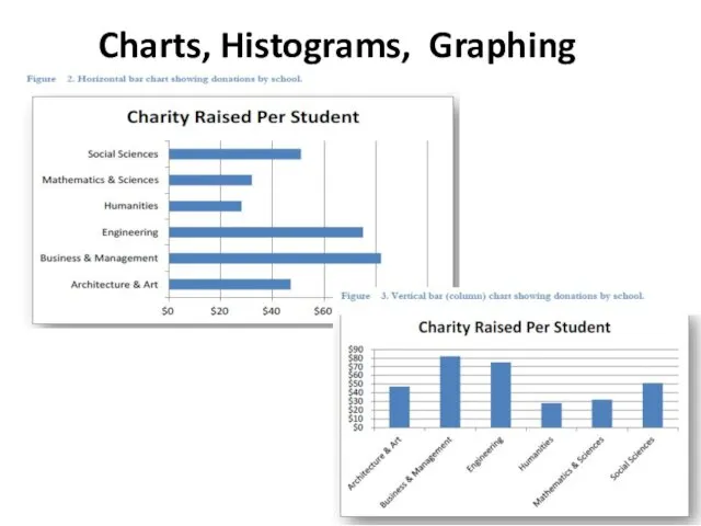
Charts, Histograms, Graphing
Charts, Histograms, Graphing
USING A HISTOGRAM TO DISPLAY
THE FREQUENCIES
The histogram displays the frequencies as
USING A HISTOGRAM TO DISPLAY
THE FREQUENCIES
The histogram displays the frequencies as
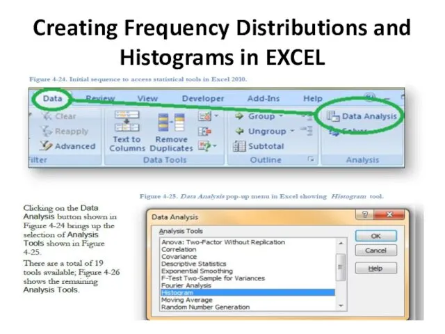
Creating Frequency Distributions and Histograms in EXCEL
Creating Frequency Distributions and Histograms in EXCEL
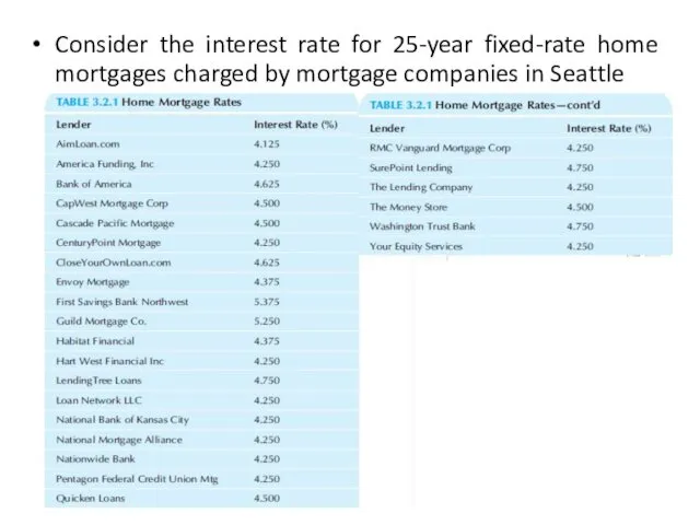
Consider the interest rate for 25-year fixed-rate home mortgages charged by
Consider the interest rate for 25-year fixed-rate home mortgages charged by


NORMAL DISTRIBUTIONS
A normal distribution is an idealized, smooth, bell-shaped histogram with
NORMAL DISTRIBUTIONS
A normal distribution is an idealized, smooth, bell-shaped histogram with

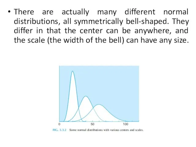
There are actually many different normal distributions, all symmetrically bell-shaped. They
There are actually many different normal distributions, all symmetrically bell-shaped. They

BIMODAL DISTRIBUTIONS WITH
TWO GROUPS
It is important to be able to recognize
BIMODAL DISTRIBUTIONS WITH
TWO GROUPS
It is important to be able to recognize
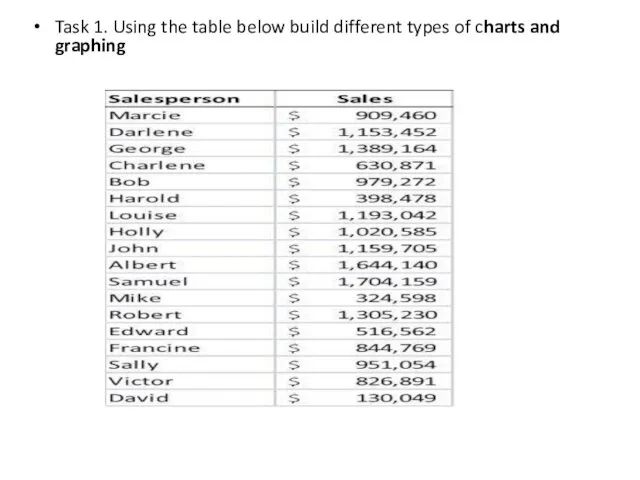
Task 1. Using the table below build different types of charts
Task 1. Using the table below build different types of charts
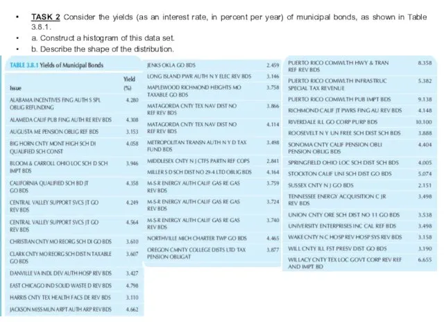
TASK 2 Consider the yields (as an interest rate, in percent
TASK 2 Consider the yields (as an interest rate, in percent
Landmark Summaries
Interpreting Typical Values and Percentiles
WHAT IS THE MOST TYPICAL VALUE?
There
Landmark Summaries
Interpreting Typical Values and Percentiles
WHAT IS THE MOST TYPICAL VALUE?
There
The Average: A Typical Value for
Quantitative Data
The average (also called the
The Average: A Typical Value for
Quantitative Data
The average (also called the

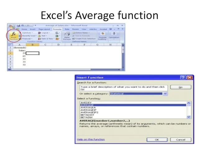
Excel’s Average function
Excel’s Average function


The Weighted Average: Adjusting
for Importance
The weighted average is like the average,
The Weighted Average: Adjusting
for Importance
The weighted average is like the average,

The Median: A Typical Value for
Quantitative and Ordinal Data
The median is
The Median: A Typical Value for
Quantitative and Ordinal Data
The median is


The Mode: A Typical Value Even
for Nominal Data
The mode is the
The Mode: A Typical Value Even
for Nominal Data
The mode is the
Example 1
The moda of the ungrouped data: 20, 18, 15, 15,
Example 1
The moda of the ungrouped data: 20, 18, 15, 15,

Task
To calculate:
The Average and The Weighted Average and Rang
1) 24,
Task
To calculate:
The Average and The Weighted Average and Rang
1) 24,
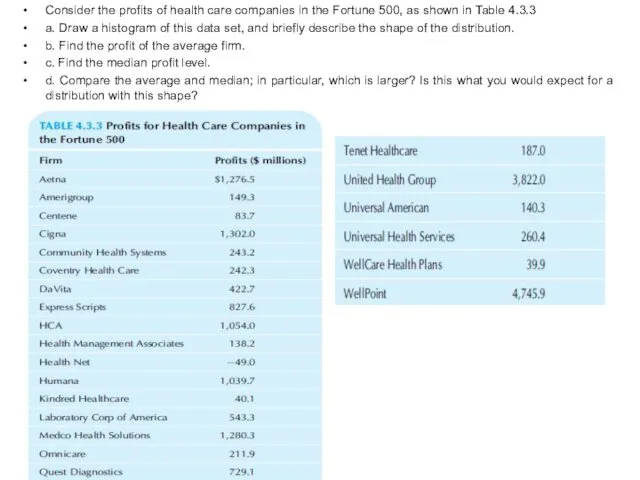
Consider the profits of health care companies in the Fortune 500,
Consider the profits of health care companies in the Fortune 500,
Task
Consider the loan fees charged for granting home mortgages,
as shown in
Task
Consider the loan fees charged for granting home mortgages,
as shown in

Probability
Understanding Random Situations
Probability is a measure quantifying the likelihood that events will
Probability
Understanding Random Situations
Probability is a measure quantifying the likelihood that events will
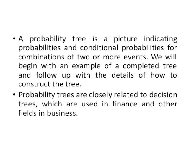
A probability tree is a picture indicating probabilities and conditional probabilities
A probability tree is a picture indicating probabilities and conditional probabilities
 Самозахист авторського права в мережі Інтернет
 НЕТ Этикет
 Классификация ИТ. Структура АИТ
 Архитектура вычислительных систем и сетей
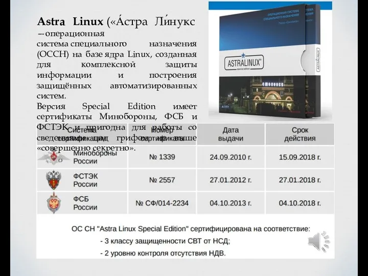 Astra Linux А́стра Ли́нукс — операционная система специального назначения
 Ms word редакторы туралы негізгі мағлұматтар
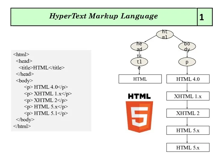 Новые элементы HyperText Markup Language
 Презентация к уроку информатики на тему: Правила поведения в компьютерном классе.
 Объявление и вызов методов в C#
 Алгоритмическая структура Цикл. Решение задач со счетчиком. 9 класс
 Introduction to computer systems. Architectures of computer systems
 The term computer programmer
 Расчет и проектировка СКС в программах Netplanner и Microsoft Office visio
 Исполнитель чертёжник
 Linux Commands
 Базы данных. Программирование баз данных
 Информационно-поисковые системы
 Компьютерный сленг
 Проектная деятельность на уроках информатики
 Информация. Понятие информации
 Проектирование АСУ. Комплекс подсистем технической подготовки производства
 Строковый тип данных Операции со строками и стандартные функции
 Учебник по Pawn программированию
 Разработка открытого урока по информатике Текстовый редактор MicrosoftWord
 Сеть и облачные технологии
 Делегаты и события в C#. Введение в язык XAML
 Личный помощник. Ввод
 Презентация Создание простых текстовых документов