- Construction and optimization of algorithms

Содержание
- 2. Literature Thomas H. Cormen Charles E. Leiserson Ronald L. Rivest Clifford Stein. Introduction to Algorithms. N.
- 3. Time complexity Тhe time complexity of the algorithm in the worst, best or average case. In
- 4. Asymptotic complexity Examples - ? Logarithmic, linear, polynomial, exponential complexity.
- 5. Other measures of complexity Other measures of complexity are also used, such as the amount of
- 6. Other measures of complexity If the created program is used only a few times, then the
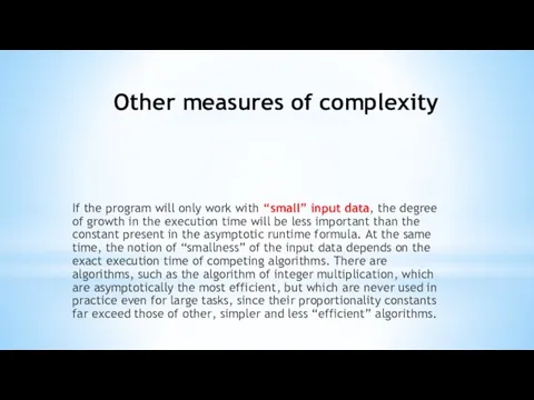
- 7. Other measures of complexity If the program will only work with “small” input data, the degree
- 8. Other measures of complexity Sometimes there are incorrect algorithms that either get looped or sometimes give
- 9. Calculate the complexity of the algorithm
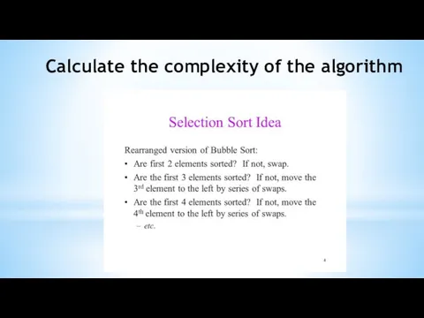
- 10. Calculate the complexity of the algorithm
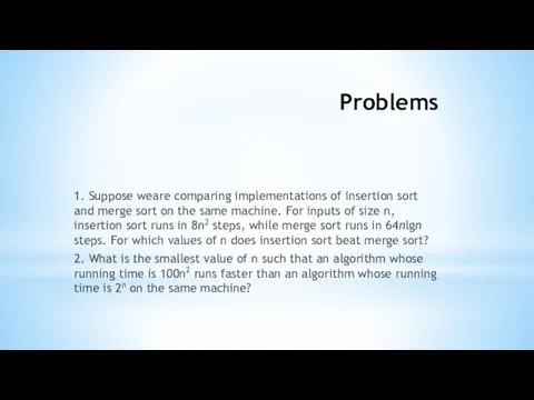
- 14. Problems 1. Suppose weare comparing implementations of insertion sort and merge sort on the same machine.
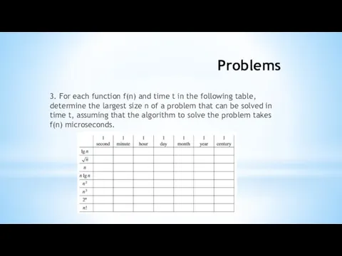
- 15. Problems 3. For each function f(n) and time t in the following table, determine the largest
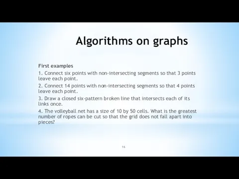
- 16. Algorithms on graphs First examples 1. Connect six points with non-intersecting segments so that 3 points
- 32. Скачать презентацию
Literature
Thomas H. Cormen Charles E. Leiserson Ronald L. Rivest Clifford Stein.
Literature
Thomas H. Cormen Charles E. Leiserson Ronald L. Rivest Clifford Stein.
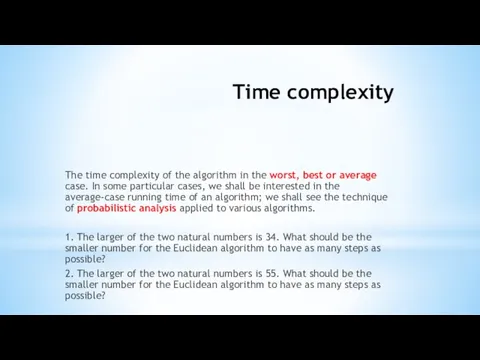
Time complexity
Тhe time complexity of the algorithm in the worst,
Time complexity
Тhe time complexity of the algorithm in the worst,
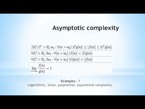
Asymptotic complexity
Examples - ?
Logarithmic, linear, polynomial, exponential complexity.
Asymptotic complexity
Examples - ?
Logarithmic, linear, polynomial, exponential complexity.

Other measures of complexity
Other measures of complexity are also used, such
Other measures of complexity
Other measures of complexity are also used, such
Other measures of complexity
If the created program is used only a
Other measures of complexity
If the created program is used only a
Other measures of complexity
If the program will only work with “small”
Other measures of complexity
If the program will only work with “small”
Other measures of complexity
Sometimes there are incorrect algorithms that either get
Other measures of complexity
Sometimes there are incorrect algorithms that either get
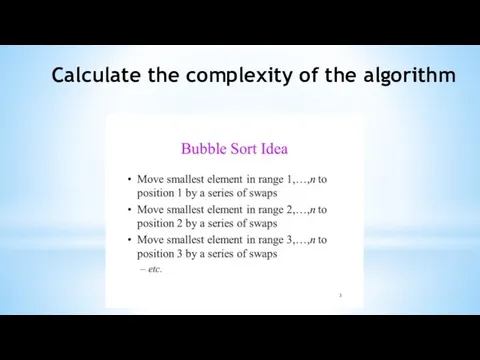
Calculate the complexity of the algorithm
Calculate the complexity of the algorithm
Calculate the complexity of the algorithm
Calculate the complexity of the algorithm
Problems
1. Suppose weare comparing implementations of insertion sort and merge sort
Problems
1. Suppose weare comparing implementations of insertion sort and merge sort
Problems
3. For each function f(n) and time t in the following
Problems
3. For each function f(n) and time t in the following
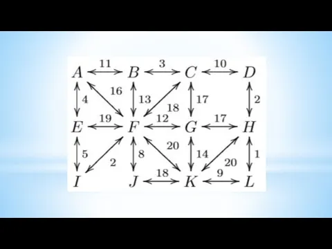
Algorithms on graphs
First examples
1. Connect six points with non-intersecting segments so
Algorithms on graphs
First examples
1. Connect six points with non-intersecting segments so


 Кодирование и обработка графической информации
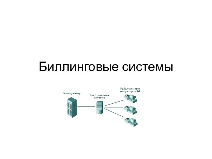 Биллинговые системы
 Техническая система. Лекция 4
 История развития компьютерной техники
 Всемирная паутина
 Информационные технологии в юридической деятельности
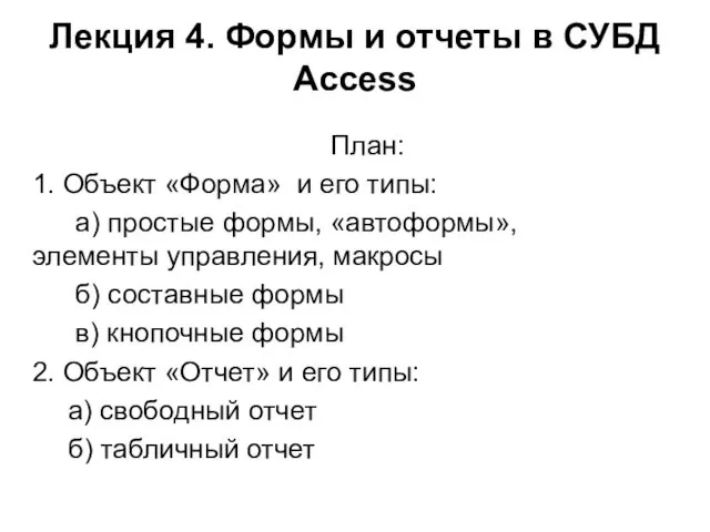 Формы и отчеты в СУБД Access
 Development of methods for determining testing strategy software systems that operate in complex computer systems
 Кибербезопасность. Индивидуальный проект
 Информационные системы как средство реализации информационных технологий. Определения. Стандарты
 Информация как объект защиты на различных уровнях её представления
 Методическая инструкция. Создание таблиц со схемами для отчета по выполненным работам
 Символьные и строковые величины. Команды ввода и вывода
 Языки программирования высокого уровня
 Использование вашего приложения
 Использование протоколов. Инкапсуляция OSI. Команды UNIX
 Оплата банковской картой
 Компьютерная графика. Урок 7
 Процесс создания дизайнерского календаря Год зайца в программе CorelDraw
 Логическая информация и основы логики
 Структурирование и классификация информации. (Тема 7)
 DS программирование
 Информация и информационные процессы
 Advantages and Disadvantages of Internet
 Файловая система. Операции с дисковыми файлами. Занятие 07
 Новый Пульт ГрузовичкоФ
 Задачи нелинейного программирования. Методы и инструментальные средства их решения
 Управление боевой подготовкой. Лекция №11