- Deep learning and rses

Содержание
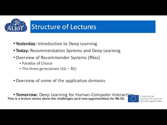
- 2. Structure of Lectures Yesterday: Introduction to Deep Learning Today: Recommendation Systems and Deep Learning Overview of
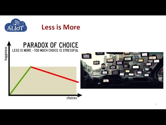
- 4. Less is More
- 5. Recommendation Systems: Academia Huge progress over the last 20 years from the 3 initial papers published
- 6. Recommender Systems in the Industry Industry pioneers: Amazon, B&N, Net Perceptions (around 1996-1997) Hello, Jim, we
- 7. Today’s Recommenders Work across many firms (Netflix, Yelp, Pandora, Google, Facebook, Twitter, LinkedIn) and they operate
- 8. Startup bought by Microsoft Co. 2011 $210millions 100 employers Buy Now or Tomorrow?
- 9. Three Generations of Recommender Systems Overview of the traditional paradigm of RSes (1st generation) Current generation
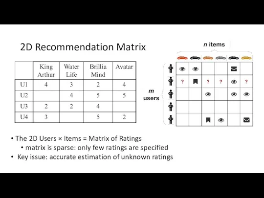
- 10. Two-dimensional (2D): Users and Items Utility of an item to a user revealed by a single
- 11. 2D Recommendation Matrix The 2D Users × Items = Matrix of Ratings matrix is sparse: only
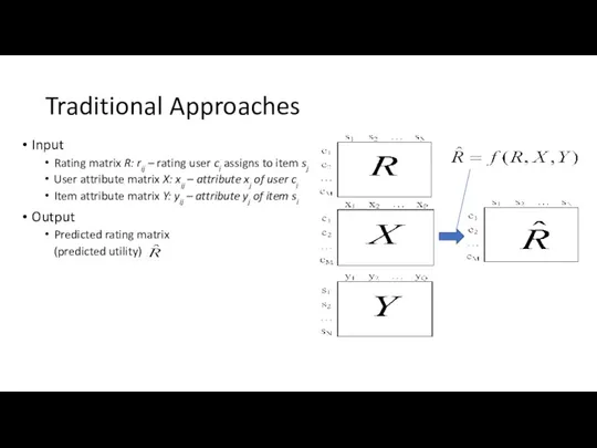
- 12. Traditional Approaches Input Rating matrix R: rij – rating user ci assigns to item sj User
- 13. Types of Recommendations [Balabanovic & Shoham 1997] Content-based build a model based on a description of
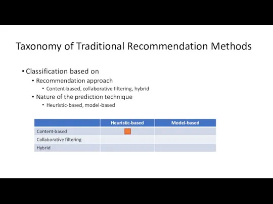
- 14. Taxonomy of Traditional Recommendation Methods Classification based on Recommendation approach Content-based, collaborative filtering, hybrid Nature of
- 15. Knowledge Discovery in Databases (KDD) process
- 16. Knowledge Discovery in Databases (KDD) process
- 17. Information Retrieval Techniques. In the KDD process, data is represented in a tabular format. There are
- 18. Item Similarity Methods: Problem No.1 In social media, individuals generate many types of nontabular data, such
- 19. Statistical Models A document is typically represented by a bag of words (unordered words with frequencies).
- 20. Boolean Model Disadvantages Similarity function is boolean Exact-match only, no partial matches Retrieved documents not ranked
- 21. Vectorization (VSM) A well-known method for vectorization is the vector-space model introduced by Salton, Wong, and
- 22. Document Collection A collection of n documents can be represented in the vector space model by
- 23. Term Weights: Inverse Document Frequency Terms that appear in many different documents are less indicative of
- 24. Term Frequency - Inverse Document Frequency (TF-IDF) In the TF-IDF scheme, wj,i is calculated as wj,i
- 25. Consider the words “apple” and “orange” that appear 10 and 20 times in document d1. Let
- 26. Consider the following three documents: d1= “social media mining” d2= “social media data” d3= “financial market
- 27. Consider the following three documents: d1= “social media mining” d2= “social media data” d3= “financial market
- 28. The IDF values are
- 29. The TF-IDF values can be computed by multiplying TF values with the IDF values: d1= “social
- 30. Item Similarity Methods Information Retrieval Techniques Item attributes correspond to word occurrences in item descriptions ,
- 31. Content-Based kNN Method Each item is defined by its content C. Content is application-specific, e.g., restaurants
- 32. Item-Based Collaborative Filtering Same rij estimation as for the user-based but use item-to-item sim(i, i’) instead
- 33. Association-Rule-Based CF Another example of CF heuristic Assume user A had transaction T with items I
- 34. Association-Rule-Based CF: Supermarket Purchases User A bought I = (Bread, Butter, Fish) Q: What else to
- 35. Hybrid: Combining Other Methods The hybrid approach can combine two or more methods to gain better
- 36. Performance Evaluation of RSes Importance of Right Metrics There are measures and… measures! Assume you improved
- 37. Evaluation Paradigms User studies Online evaluations (A/B tests) Offline evaluation with observational data Long-term goals vs.
- 38. Example of A/B Testing Online University: a RS recommends remedial learning materials to the students who
- 39. Accuracy-Based Metrics For Prediction RMSE and MAE For Classification Precision: percentage of good recommendations among all
- 40. Netflix Prize Competition Competition for the best algorithm to predict user ratings for films based on
- 41. Test Set Results (RMSE) The Ensemble: 0.856714 BellKor’s Pragmatic Theory: 0.856704 Both scores round to 0.8567
- 42. What Netflix Prize Winners Done Development of new and scalable methods, MF being the most prominent
- 43. Netflix Competition: The End of an Era Netflix Prize Competition: Completed not only the 2D, but
- 44. Thinking Outside of the 3MR Box The 3MR paradigm worked well for Netflix. But what about
- 45. Context-Aware Recommender Systems (CARS) Recommend a vacation Winter vs. summer Recommend a movie To a student
- 46. What is Context in Recommender Systems A multifaceted concept: 150 (!) definitions from various disciplines (Bazire&Brezillon
- 47. Context-Aware Recommendation Problem Data in context-aware recommender systems (CARS) Rating information: In addition to information about
- 48. How to Use Context in Recommender Systems [AT10] Context can be used in the following stages
- 49. Paradigms for Incorporating Context in Recommender Systems [AT08]
- 50. Multidimensional Recommender Systems Traditional 2D Matrix Multidimensional (OLAP-based) cube Problem: how to estimate ratings on this
- 51. Mobile Recommender Systems A special case of CARS Very different from traditional RSes Spatial context Temporal
- 52. Route Recommendations for Taxi Drivers (based on [Ge et al 2010]) Goal: recommend travel routes to
- 53. Key Ideas Behind the Solution Need to model/represent driving routes Finite set of popular/historical “pick up
- 54. Results of a Study Data on 500 taxis in SF driving over 30 days “Successful” drivers:
- 55. Why DL for RSes? ImageNet challenge error rates (red line = human performance)
- 56. DL for Vehicle Recommendations Using deep learning to improve vehicle suggestions, we have two basic goals:
- 57. Preference Prediction Model The overall network consists of three subnetworks: UserNet, ItemNet and RankNet. These networks
- 58. Candidate Generation To quickly find candidates that are likely to be relevant for a user, we
- 59. Ranking For T item candidates for our user, we can use the RankNet to score each
- 60. Deep content-based music recommendation Pioneer work from Spotify also uses CNNs to extract audio features from
- 61. Is deeper better? For image classification deeper models with hundreds of layers and novel architecture shave
- 62. Unexpected & Serendipitous RSes
- 63. “A world constructed from the familiar is a world in which there’s nothing to learn ...
- 64. The Filter Bubble Example Problem with accuracy: can lead to boring recommendations
- 65. Serendipity and Unexpectedness: Breaking out of the Filter Bubble Serendipity: Recommendations of novel items liked by
- 66. Definition of Unexpectedness “If you do not expect it, you will not find the unexpected, for
- 67. Examples of Unexpected Recommendations Recommendations User Profile
- 68. Expected Recommendations Examples of sets of user expectations Expectation set of a user: a finite collection
- 69. Operationalization of Unexpectedness
- 70. Utility of Recommendations
- 71. Unexpectedness and the Long Tail The “rich gets richer” problem of RSes (a.k.a. the “blockbuster” phenomenon)
- 72. Tomorrow: Deep Learning for Human-Computer Interaction
- 74. Скачать презентацию
Structure of Lectures
Yesterday: Introduction to Deep Learning
Today: Recommendation Systems and Deep
Structure of Lectures
Yesterday: Introduction to Deep Learning
Today: Recommendation Systems and Deep
Less is More
Less is More
Recommendation Systems: Academia
Huge progress over the last 20 years
from the
Recommendation Systems: Academia
Huge progress over the last 20 years
from the
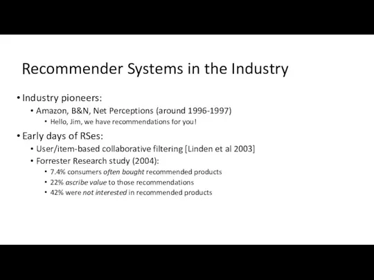
Recommender Systems in the Industry
Industry pioneers:
Amazon, B&N, Net Perceptions (around 1996-1997)
Hello,
Recommender Systems in the Industry
Industry pioneers:
Amazon, B&N, Net Perceptions (around 1996-1997)
Hello,
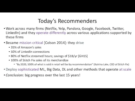
Today’s Recommenders
Work across many firms (Netflix, Yelp, Pandora, Google, Facebook, Twitter,
Today’s Recommenders
Work across many firms (Netflix, Yelp, Pandora, Google, Facebook, Twitter,
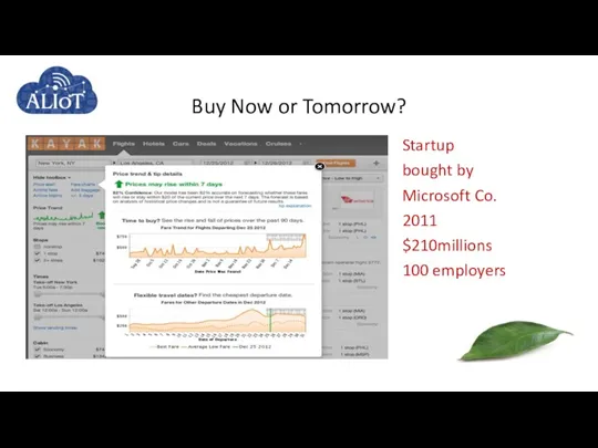
Startup
bought by
Microsoft Co.
2011
$210millions
100 employers
Buy Now or Tomorrow?
Startup
bought by
Microsoft Co.
2011
$210millions
100 employers
Buy Now or Tomorrow?
Three Generations of Recommender Systems
Overview of the traditional paradigm of RSes
Three Generations of Recommender Systems
Overview of the traditional paradigm of RSes
Two-dimensional (2D): Users and Items
Utility of an item to a user
Two-dimensional (2D): Users and Items
Utility of an item to a user
2D Recommendation Matrix
The 2D Users × Items = Matrix of
2D Recommendation Matrix
The 2D Users × Items = Matrix of
Traditional Approaches
Input
Rating matrix R: rij – rating user ci assigns to
Traditional Approaches
Input
Rating matrix R: rij – rating user ci assigns to
![Types of Recommendations [Balabanovic & Shoham 1997] Content-based build a](/_ipx/f_webp&q_80&fit_contain&s_1440x1080/imagesDir/jpg/3469/slide-12.jpg)
Types of Recommendations [Balabanovic & Shoham 1997]
Content-based
build a model based on
Types of Recommendations [Balabanovic & Shoham 1997]
Content-based
build a model based on
Taxonomy of Traditional Recommendation Methods
Classification based on
Recommendation approach
Content-based, collaborative filtering,
Taxonomy of Traditional Recommendation Methods
Classification based on
Recommendation approach
Content-based, collaborative filtering,
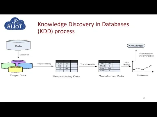
Knowledge Discovery in Databases (KDD) process
Knowledge Discovery in Databases (KDD) process
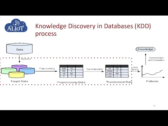
Knowledge Discovery in Databases (KDD) process
Knowledge Discovery in Databases (KDD) process
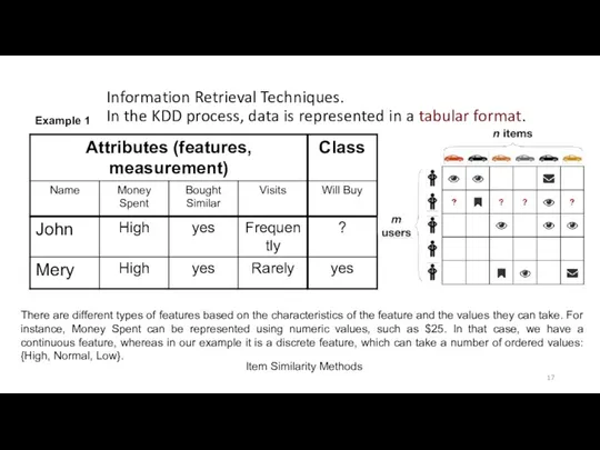
Information Retrieval Techniques.
In the KDD process, data is represented in
Information Retrieval Techniques. In the KDD process, data is represented in
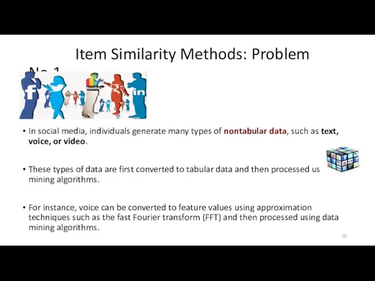
Item Similarity Methods: Problem No.1
In social media, individuals generate many
Item Similarity Methods: Problem No.1
In social media, individuals generate many
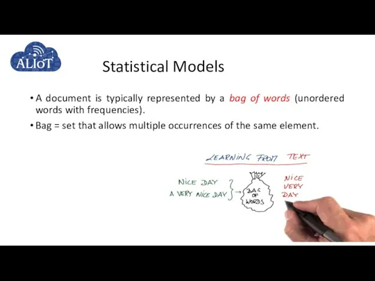
Statistical Models
A document is typically represented by a bag of
Statistical Models
A document is typically represented by a bag of
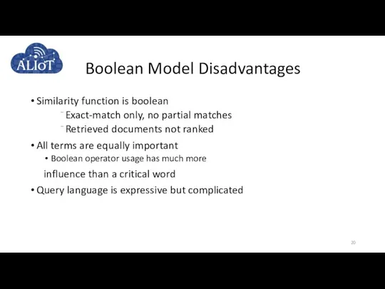
Boolean Model Disadvantages
Similarity function is boolean
Exact-match only, no partial matches
Retrieved
Boolean Model Disadvantages
Similarity function is boolean
Exact-match only, no partial matches
Retrieved
Vectorization (VSM)
A well-known method for vectorization is the vector-space model introduced
Vectorization (VSM)
A well-known method for vectorization is the vector-space model introduced
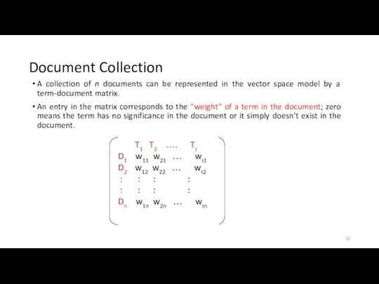
Document Collection
A collection of n documents can be represented in the
Document Collection
A collection of n documents can be represented in the
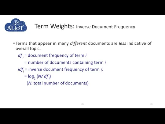
Term Weights: Inverse Document Frequency
Terms that appear in many different
Term Weights: Inverse Document Frequency
Terms that appear in many different
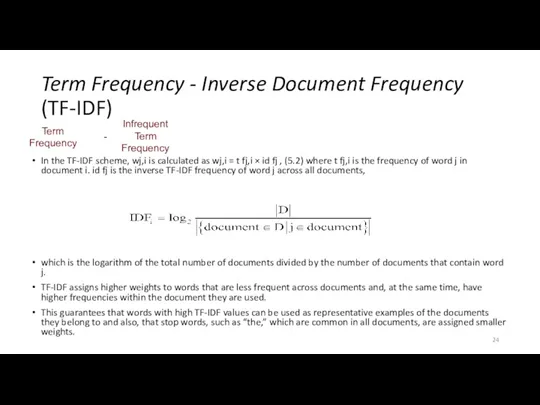
Term Frequency - Inverse Document Frequency (TF-IDF)
In the TF-IDF scheme,
Term Frequency - Inverse Document Frequency (TF-IDF)
In the TF-IDF scheme,
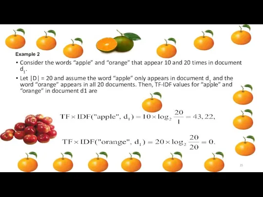
Consider the words “apple” and “orange” that appear 10 and 20
Consider the words “apple” and “orange” that appear 10 and 20
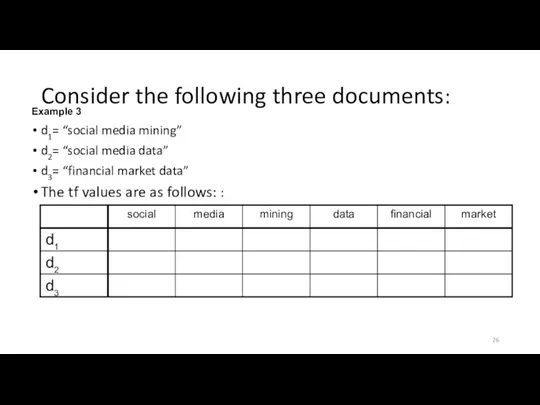
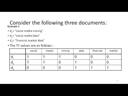
Consider the following three documents:
d1= “social media mining”
d2= “social media data”
d3=
Consider the following three documents:
d1= “social media mining”
d2= “social media data”
d3=
Consider the following three documents:
d1= “social media mining”
d2= “social media data”
d3=
Consider the following three documents:
d1= “social media mining”
d2= “social media data”
d3=
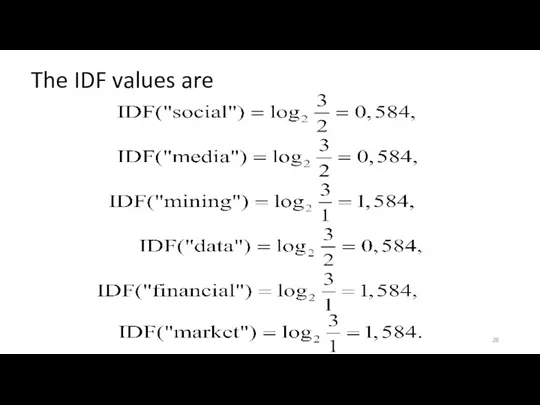
The IDF values are
The IDF values are
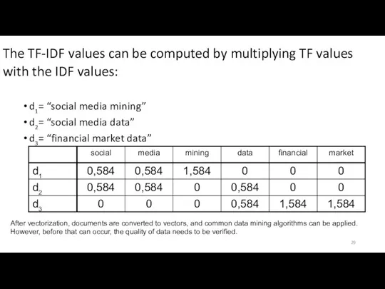
The TF-IDF values can be computed by multiplying TF values with
The TF-IDF values can be computed by multiplying TF values with
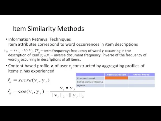
Item Similarity Methods
Information Retrieval Techniques
Item attributes correspond to word occurrences in
Item Similarity Methods
Information Retrieval Techniques Item attributes correspond to word occurrences in
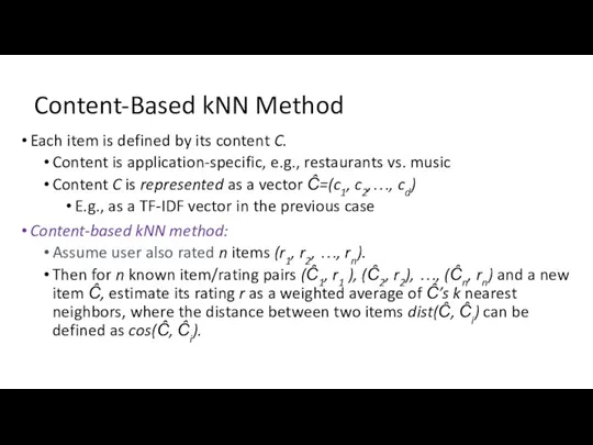
Content-Based kNN Method
Each item is defined by its content C.
Content is
Content-Based kNN Method
Each item is defined by its content C.
Content is
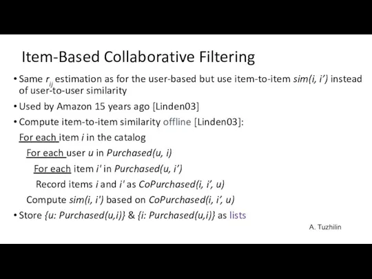
Item-Based Collaborative Filtering
Same rij estimation as for the user-based but use
Item-Based Collaborative Filtering
Same rij estimation as for the user-based but use
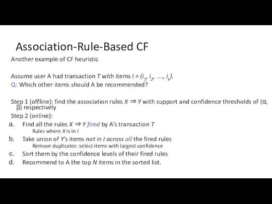
Association-Rule-Based CF
Another example of CF heuristic
Assume user A had transaction T
Association-Rule-Based CF
Another example of CF heuristic
Assume user A had transaction T
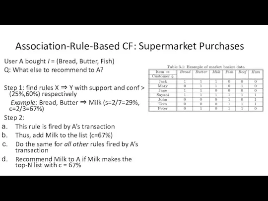
Association-Rule-Based CF: Supermarket Purchases
User A bought I = (Bread, Butter, Fish)
Q:
Association-Rule-Based CF: Supermarket Purchases
User A bought I = (Bread, Butter, Fish)
Q:
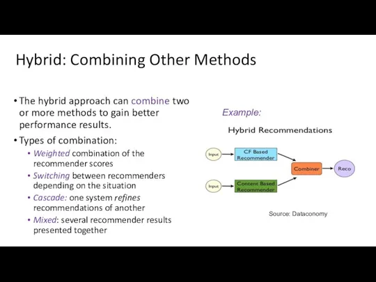
Hybrid: Combining Other Methods
The hybrid approach can combine two or more
Hybrid: Combining Other Methods
The hybrid approach can combine two or more
Performance Evaluation of RSes
Importance of Right Metrics
There are measures and… measures!
Assume
Performance Evaluation of RSes
Importance of Right Metrics
There are measures and… measures!
Assume
Evaluation Paradigms
User studies
Online evaluations (A/B tests)
Offline evaluation with observational data
Long-term goals
Evaluation Paradigms
User studies
Online evaluations (A/B tests)
Offline evaluation with observational data
Long-term goals
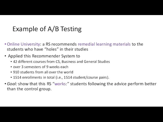
Example of A/B Testing
Online University: a RS recommends remedial learning materials
Example of A/B Testing
Online University: a RS recommends remedial learning materials
Accuracy-Based Metrics
For Prediction
RMSE and MAE
For Classification
Precision: percentage of good recommendations among
Accuracy-Based Metrics
For Prediction
RMSE and MAE
For Classification
Precision: percentage of good recommendations among
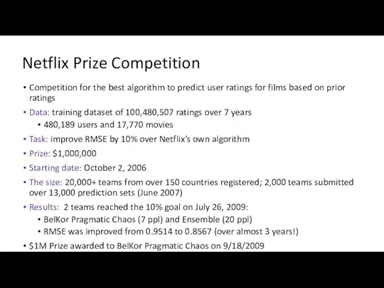
Netflix Prize Competition
Competition for the best algorithm to predict user ratings
Netflix Prize Competition
Competition for the best algorithm to predict user ratings
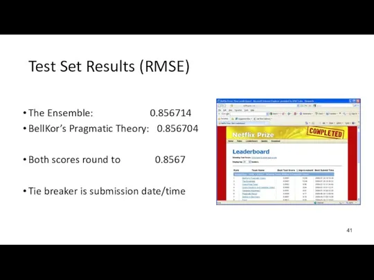
Test Set Results (RMSE)
The Ensemble: 0.856714
BellKor’s Pragmatic Theory: 0.856704
Both scores round
Test Set Results (RMSE)
The Ensemble: 0.856714
BellKor’s Pragmatic Theory: 0.856704
Both scores round
What Netflix Prize Winners Done
Development of new and scalable methods, MF
What Netflix Prize Winners Done
Development of new and scalable methods, MF
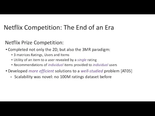
Netflix Competition: The End of an Era
Netflix Prize Competition:
Completed not
Netflix Competition: The End of an Era
Netflix Prize Competition:
Completed not
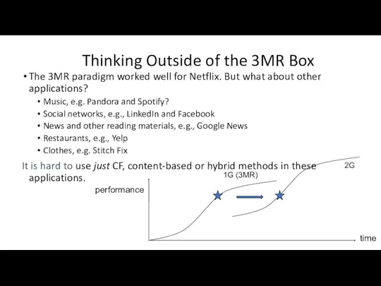
Thinking Outside of the 3MR Box
The 3MR paradigm worked well for
Thinking Outside of the 3MR Box
The 3MR paradigm worked well for
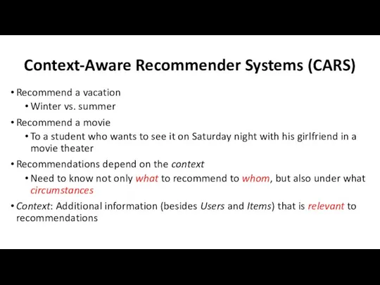
Context-Aware Recommender Systems (CARS)
Recommend a vacation
Winter vs. summer
Recommend a movie
To
Context-Aware Recommender Systems (CARS)
Recommend a vacation
Winter vs. summer
Recommend a movie
To
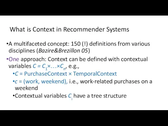
What is Context in Recommender Systems
A multifaceted concept: 150 (!) definitions
What is Context in Recommender Systems
A multifaceted concept: 150 (!) definitions
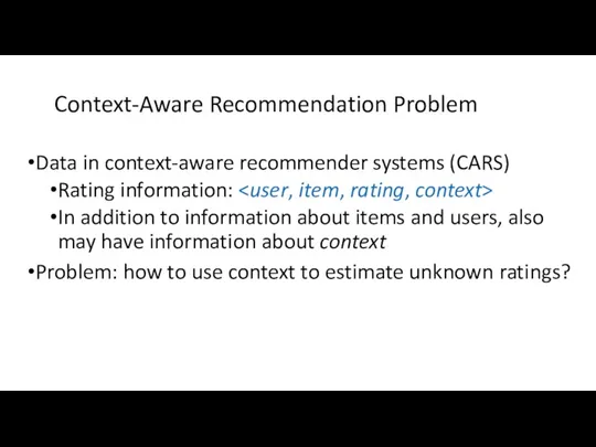
Context-Aware Recommendation Problem
Data in context-aware recommender systems (CARS)
Rating information:
Context-Aware Recommendation Problem
Data in context-aware recommender systems (CARS)
Rating information:
![How to Use Context in Recommender Systems [AT10] Context can](/_ipx/f_webp&q_80&fit_contain&s_1440x1080/imagesDir/jpg/3469/slide-47.jpg)
How to Use Context in Recommender Systems [AT10]
Context can be used
How to Use Context in Recommender Systems [AT10]
Context can be used
![Paradigms for Incorporating Context in Recommender Systems [AT08]](/_ipx/f_webp&q_80&fit_contain&s_1440x1080/imagesDir/jpg/3469/slide-48.jpg)
Paradigms for Incorporating Context in Recommender Systems [AT08]
Paradigms for Incorporating Context in Recommender Systems [AT08]
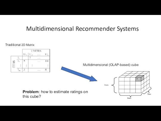
Multidimensional Recommender Systems
Traditional 2D Matrix
Multidimensional (OLAP-based) cube
Problem: how to estimate ratings
Multidimensional Recommender Systems
Traditional 2D Matrix
Multidimensional (OLAP-based) cube
Problem: how to estimate ratings
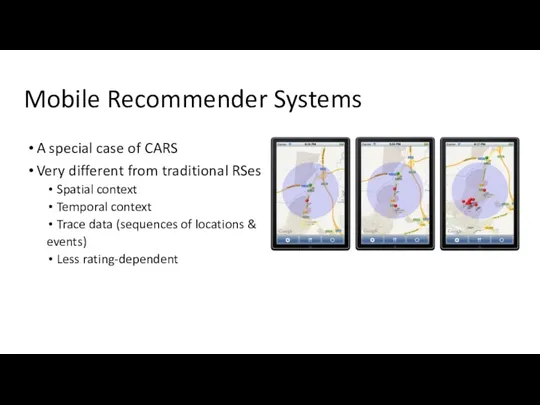
Mobile Recommender Systems
A special case of CARS
Very different from traditional RSes
Spatial
Mobile Recommender Systems
A special case of CARS
Very different from traditional RSes
Spatial
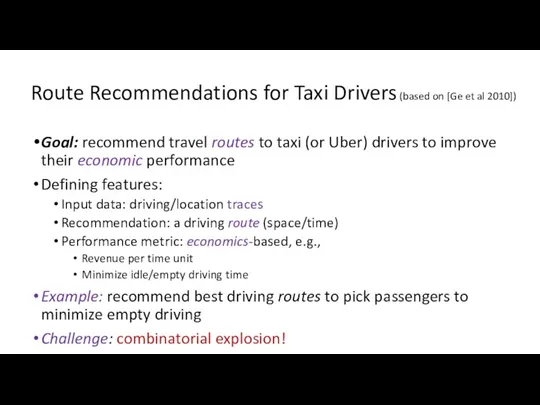
Route Recommendations for Taxi Drivers (based on [Ge et al 2010])
Goal:
Route Recommendations for Taxi Drivers (based on [Ge et al 2010])
Goal:
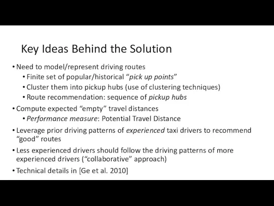
Key Ideas Behind the Solution
Need to model/represent driving routes
Finite set of
Key Ideas Behind the Solution
Need to model/represent driving routes
Finite set of
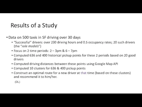
Results of a Study
Data on 500 taxis in SF driving over
Results of a Study
Data on 500 taxis in SF driving over
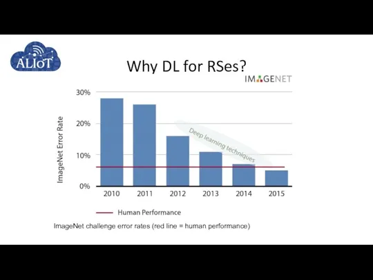
Why DL for RSes?
ImageNet challenge error rates (red line = human
Why DL for RSes?
ImageNet challenge error rates (red line = human
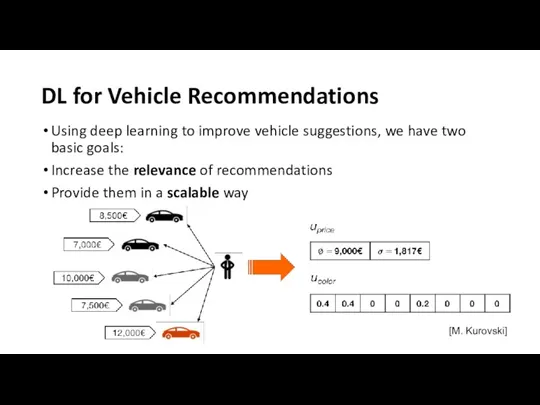
DL for Vehicle Recommendations
Using deep learning to improve vehicle suggestions, we
DL for Vehicle Recommendations
Using deep learning to improve vehicle suggestions, we
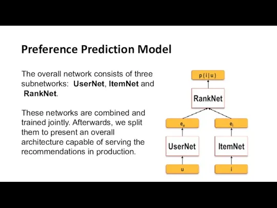
Preference Prediction Model
The overall network consists of three subnetworks: UserNet, ItemNet and RankNet.
Preference Prediction Model
The overall network consists of three subnetworks: UserNet, ItemNet and RankNet.
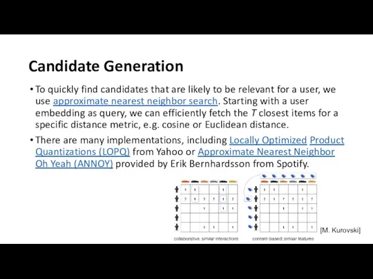
Candidate Generation
To quickly find candidates that are likely to be relevant
Candidate Generation
To quickly find candidates that are likely to be relevant
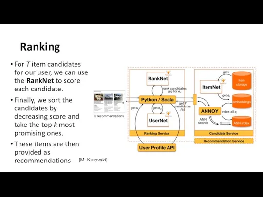
Ranking
For T item candidates for our user, we can use the RankNet to score each
Ranking
For T item candidates for our user, we can use the RankNet to score each
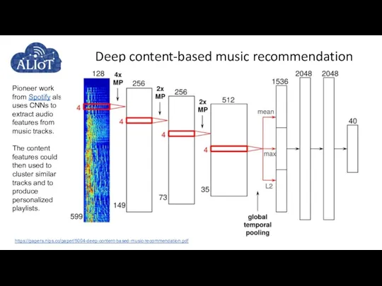
Deep content-based music recommendation
Pioneer work from Spotify also uses CNNs to extract audio
Deep content-based music recommendation
Pioneer work from Spotify also uses CNNs to extract audio
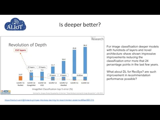
Is deeper better?
For image classification deeper models with hundreds of layers
Is deeper better?
For image classification deeper models with hundreds of layers
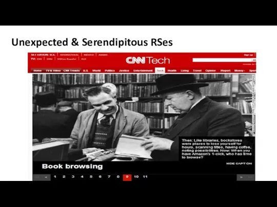
Unexpected & Serendipitous RSes
Unexpected & Serendipitous RSes
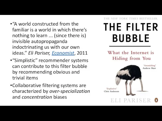
“A world constructed from the familiar is a world in which
“A world constructed from the familiar is a world in which
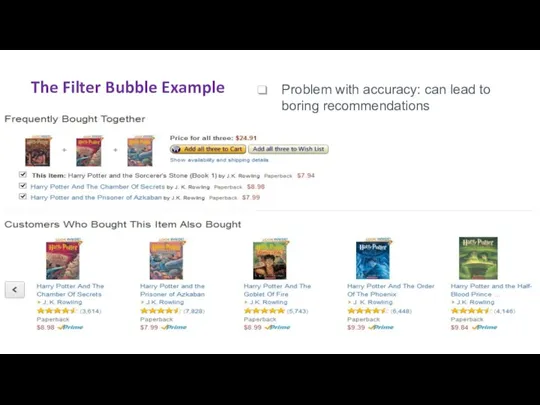
The Filter Bubble Example
Problem with accuracy: can lead to boring recommendations
The Filter Bubble Example
Problem with accuracy: can lead to boring recommendations
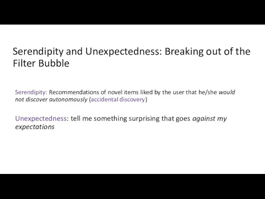
Serendipity and Unexpectedness: Breaking out of the Filter Bubble
Serendipity: Recommendations of
Serendipity and Unexpectedness: Breaking out of the Filter Bubble
Serendipity: Recommendations of
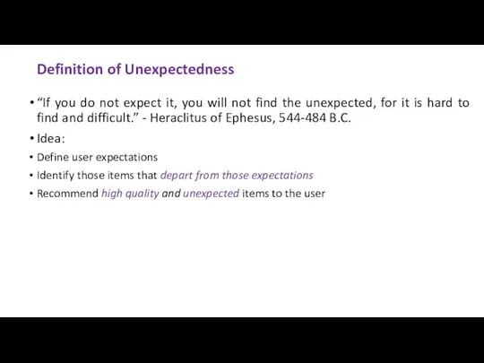
Definition of Unexpectedness
“If you do not expect it, you will not
Definition of Unexpectedness
“If you do not expect it, you will not
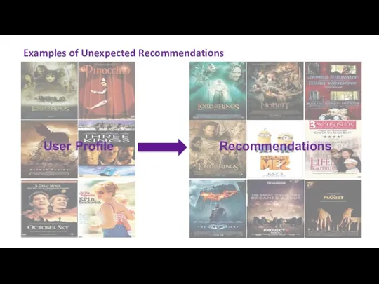
Examples of Unexpected Recommendations
Recommendations
User Profile
Examples of Unexpected Recommendations
Recommendations
User Profile
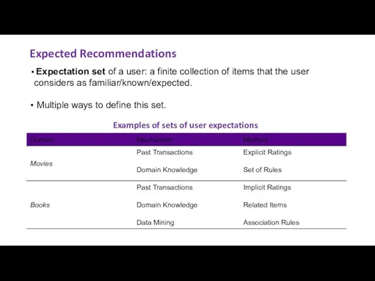
Expected Recommendations
Examples of sets of user expectations
Expectation set of a
Expected Recommendations
Examples of sets of user expectations
Expectation set of a
Operationalization of Unexpectedness
Operationalization of Unexpectedness
Utility of Recommendations
Utility of Recommendations
Unexpectedness and the Long Tail
The “rich gets richer” problem of RSes
Unexpectedness and the Long Tail
The “rich gets richer” problem of RSes
Tomorrow: Deep Learning for Human-Computer Interaction
Tomorrow: Deep Learning for Human-Computer Interaction
 Диалоги и диалоговые окна. Диалоговые окна Windows
 Интернет и его службы
 Вкладені алгоритмічні структури розгалуження. Вкладені розгалуження
 Работа с электронными таблицами в программе Microsoft Excel
 Программирование на алгоритмическом языке (7 класс)
 Сопровождение информационных систем
 Ғаламтор желісінің қоғам өміріндегі орны атты тақырыптағы ғылыми жобасы
 Продвижение здорового образа жизни в массы с помощью инфотеймента. Проект
 Інформаційні технології у навчанні
 Лекция №15 Web, JSON
 Нормальные формы
 Массивы. Операции с массивами
 Разбор задач ЕГЭ. Системы счисления
 Информационное покрытие НПАО Светогорский ЦБК в СМИ и медиа
 Кодирование звуковой и видеоинформации
 Компания DNS (Digital Network System
 Построение диаграмм и графиков в электронных таблицах
 Мошенничества в интернет
 Коммуникативная природа информационного общества. Определение коммуникации
 Двумерные массивы. Действия со строками и столбцами.
 Характеристика областей знаний по инженерии программного обеспечения — SWEBOK
 Расчетные методики ПП ЭкоСфера-предприятие. Расчет выбросов из резервуаров
 Главные тренды
 Среда программирования QBASIK
 Компьютерные презентации
 Операционная система Windows Vista
 Задание по информатике №19 - №21
 Нашествие. 8 эпизод