- System analysis and decision making Decision Trees

Содержание
- 2. The systematic use of trees for knowledge representation can be used for fast and frugal decisions.
- 3. Bayesian model System analysis and decision making
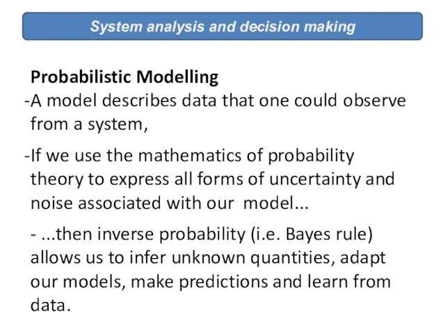
- 4. System analysis and decision making Probabilistic Modelling A model describes data that one could observe from
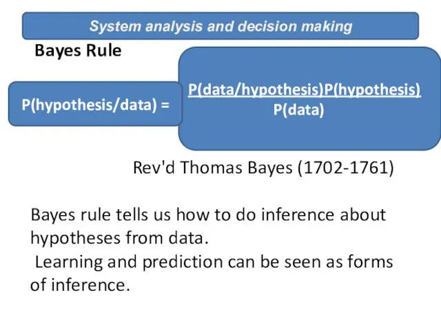
- 5. System analysis and decision making Bayes Rule Rev'd Thomas Bayes (1702-1761) Bayes rule tells us how
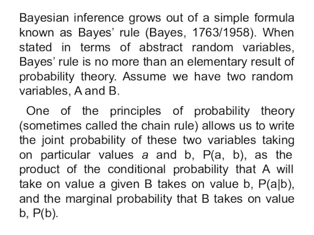
- 6. Bayesian inference grows out of a simple formula known as Bayes’ rule (Bayes, 1763/1958). When stated
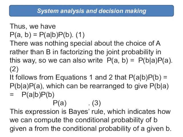
- 7. System analysis and decision making Thus, we have P(a, b) = P(a|b)P(b). (1) There was nothing
- 8. System analysis and decision making The both full Bayesian inference and one-reason decision making are processes
- 9. Subtrees of the full tree not containing any path from a root to leaves are regarded
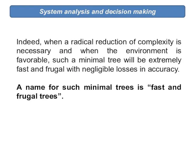
- 10. System analysis and decision making Indeed, when a radical reduction of complexity is necessary and when
- 11. System analysis and decision making TREE-STRUCTURED REPRESENTATIONS IN CLASSIFICATION TASKS
- 12. System analysis and decision making Human classifications and decisions are based on the analysis of features
- 13. System analysis and decision making Among the diverse representation a device for classification, trees have been
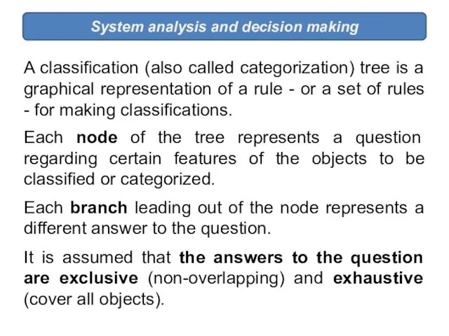
- 14. System analysis and decision making A classification (also called categorization) tree is a graphical representation of
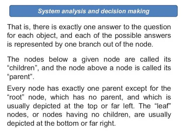
- 15. System analysis and decision making That is, there is exactly one answer to the question for
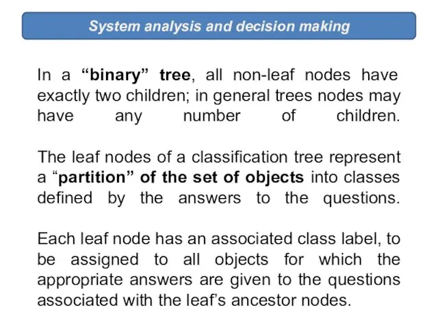
- 16. In a “binary” tree, all non-leaf nodes have exactly two children; in general trees nodes may
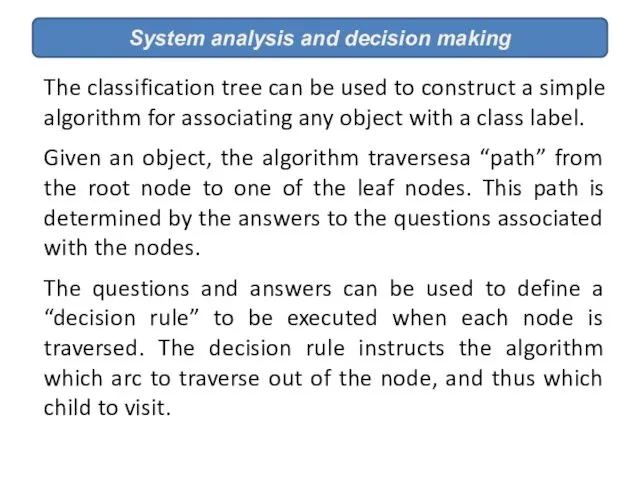
- 17. System analysis and decision making The classification tree can be used to construct a simple algorithm
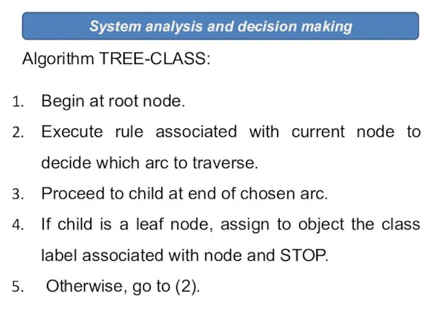
- 18. System analysis and decision making Algorithm TREE-CLASS: Begin at root node. Execute rule associated with current
- 19. System analysis and decision making Natural Frequency Trees Natural frequency trees provide good representations of the
- 20. System analysis and decision making
- 21. Figures 1. The natural frequency tree for classifying a patient as having or not having cancer,
- 22. How many of the women who get a positive mammography and a positive ultrasound test do
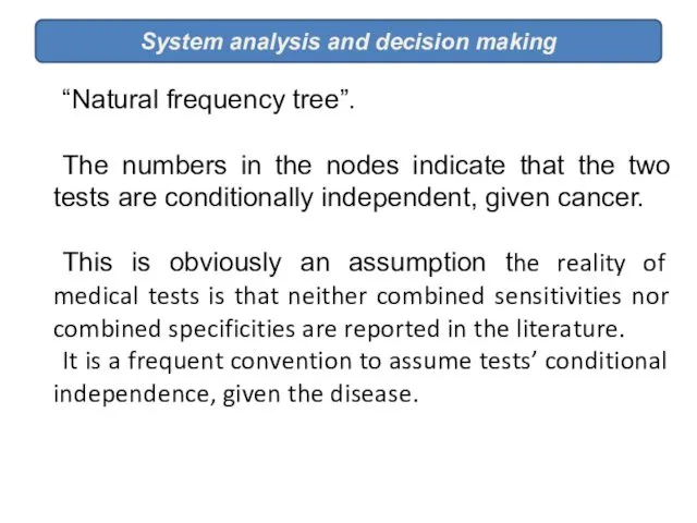
- 23. System analysis and decision making “Natural frequency tree”. The numbers in the nodes indicate that the
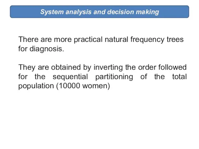
- 24. System analysis and decision making There are more practical natural frequency trees for diagnosis. They are
- 25. Figures 2. The natural frequency tree obtained from the tree, when the sampling order is mammogram
- 26. Organizing the tree in the diagnostic direction produces a much more efficient classification strategy. This tree
- 27. System analysis and decision making Second, once we have placed a patient at a node just
- 28. That is, the probability comparing the leaves of Figures 1 and 2 reveals that they are
- 29. System analysis and decision making Knowledge tends to be organised causally, and diagnostic inference is performed
- 30. System analysis and decision making However, ecologically situated agents tend to adopt representations tailored to their
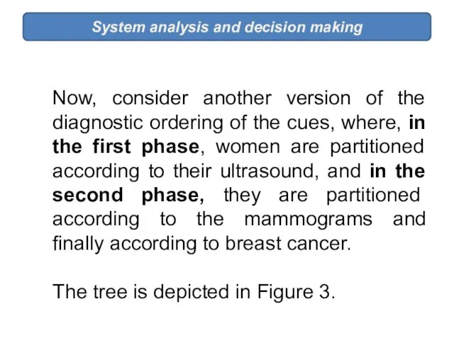
- 31. System analysis and decision making Now, consider another version of the diagnostic ordering of the cues,
- 32. Figure 3. Natural sampling in the order ultrasound → mammography → cancer our hypothetical woman has
- 33. System analysis and decision making FAST AND FRUGAL TREES A tree may be called a fast
- 34. System analysis and decision making An important convention has to be applied beforehand: cue profiles can
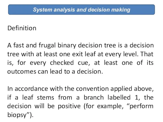
- 35. System analysis and decision making Definition A fast and frugal binary decision tree is a decision
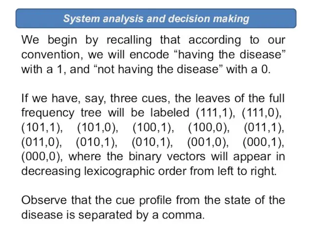
- 36. System analysis and decision making We begin by recalling that according to our convention, we will
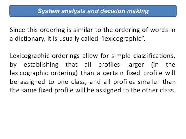
- 37. System analysis and decision making Since this ordering is similar to the ordering of words in
- 38. A lexicographic classifier determined by the path of profile (101), where the three bits are cue
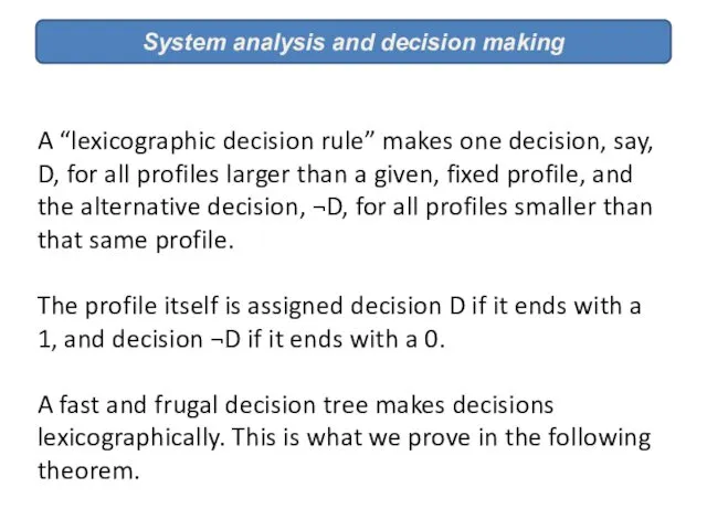
- 39. System analysis and decision making A “lexicographic decision rule” makes one decision, say, D, for all
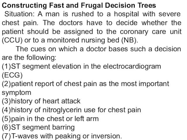
- 40. Constructing Fast and Frugal Decision Trees Situation: A man is rushed to a hospital with severe
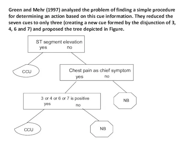
- 41. Green and Mehr (1997) analyzed the problem of finding a simple procedure for determining an action
- 42. System analysis and decision making Although Green and Mehr (1997) succeeded in constructing a fast and
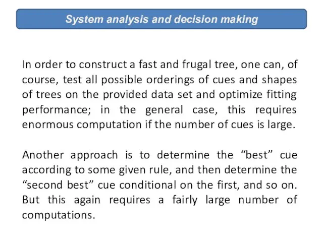
- 43. System analysis and decision making In order to construct a fast and frugal tree, one can,
- 44. System analysis and decision making In conceptual analogy to Bayes models, decision makers will not look
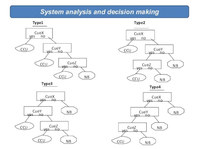
- 45. System analysis and decision making The Shape of Trees There are four possible shapes, or branching
- 46. System analysis and decision making
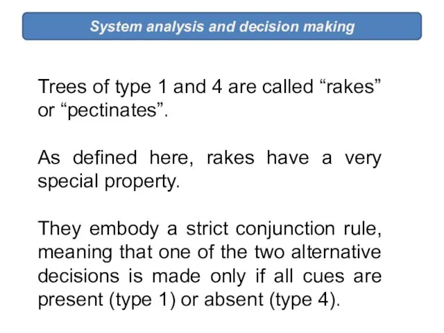
- 47. System analysis and decision making Trees of type 1 and 4 are called “rakes” or “pectinates”.
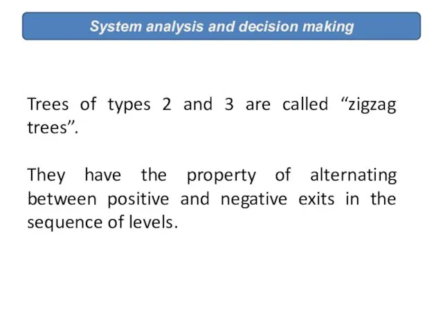
- 48. System analysis and decision making Trees of types 2 and 3 are called “zigzag trees”. They
- 49. System analysis and decision making Cue interactions go beyond the bivariate contingencies that are typically observed
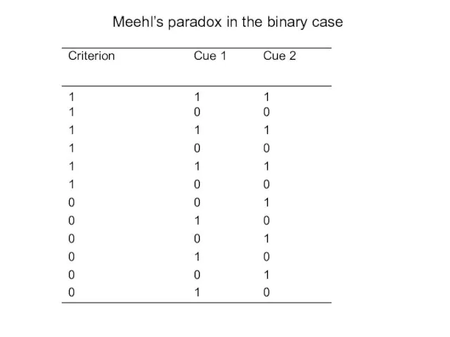
- 50. Meehl’s paradox in the binary case
- 51. The “paradoxical” nature of the given example is due to the fact that both single cues
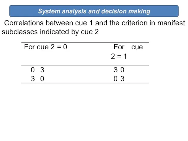
- 52. System analysis and decision making Correlations between cue 1 and the criterion in manifest subclasses indicated
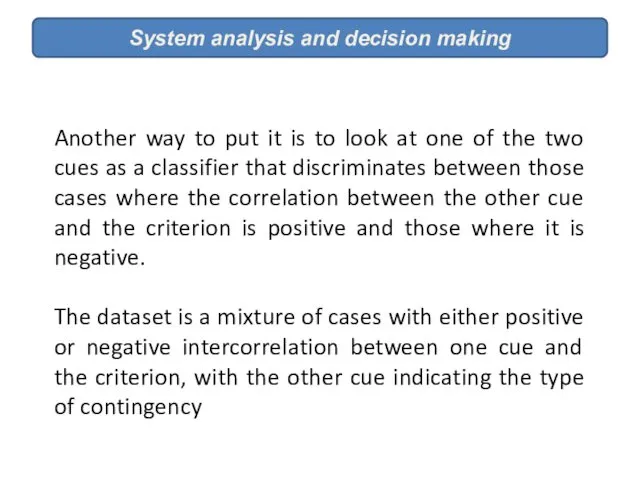
- 53. System analysis and decision making Another way to put it is to look at one of
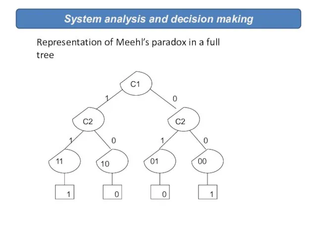
- 54. System analysis and decision making Representation of Meehl’s paradox in a full tree
- 55. System analysis and decision making Simple trees bet on a certain structure of the world, irrespective
- 56. System analysis and decision making From a statistical point of view, it would, of course, be
- 57. System analysis and decision making For instance, even for large epidemiological trials in medicine, it often
- 58. System analysis and decision making The fact that cue interactions can exist, and that they can
- 60. Скачать презентацию
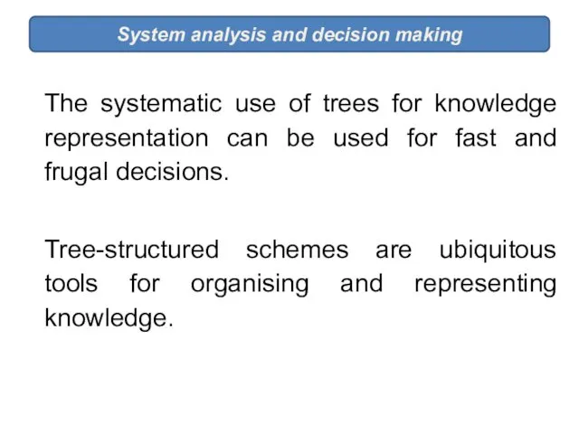
The systematic use of trees for knowledge representation can be
The systematic use of trees for knowledge representation can be
Bayesian model
System analysis and decision making
Bayesian model
System analysis and decision making
System analysis and decision making
Probabilistic Modelling
A model describes data that
System analysis and decision making
Probabilistic Modelling
A model describes data that
System analysis and decision making
Bayes Rule
Rev'd Thomas Bayes
System analysis and decision making
Bayes Rule
Rev'd Thomas Bayes
Bayesian inference grows out of a simple formula known as
Bayesian inference grows out of a simple formula known as
System analysis and decision making
Thus, we have
P(a, b) = P(a|b)P(b).
System analysis and decision making
Thus, we have
P(a, b) = P(a|b)P(b).
System analysis and decision making
The both full Bayesian inference and
System analysis and decision making
The both full Bayesian inference and
Subtrees of the full tree not containing any path from
Subtrees of the full tree not containing any path from
System analysis and decision making
Indeed, when a radical reduction of
System analysis and decision making
Indeed, when a radical reduction of
System analysis and decision making
TREE-STRUCTURED REPRESENTATIONS IN CLASSIFICATION TASKS
System analysis and decision making
TREE-STRUCTURED REPRESENTATIONS IN CLASSIFICATION TASKS
System analysis and decision making
Human classifications and decisions are based
System analysis and decision making
Human classifications and decisions are based
System analysis and decision making
Among the diverse representation a device
System analysis and decision making
Among the diverse representation a device
System analysis and decision making
A classification (also called categorization) tree
System analysis and decision making
A classification (also called categorization) tree
System analysis and decision making
That is, there is exactly one
System analysis and decision making
That is, there is exactly one
In a “binary” tree, all non-leaf nodes have exactly two children;
In a “binary” tree, all non-leaf nodes have exactly two children;
System analysis and decision making
The classification tree can be used
System analysis and decision making
The classification tree can be used
System analysis and decision making
Algorithm TREE-CLASS:
Begin at root node.
Execute rule
System analysis and decision making
Algorithm TREE-CLASS:
Begin at root node.
Execute rule
System analysis and decision making
Natural Frequency Trees
Natural frequency trees provide
System analysis and decision making
Natural Frequency Trees
Natural frequency trees provide
System analysis and decision making
System analysis and decision making
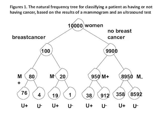
Figures 1. The natural frequency tree for classifying a patient
Figures 1. The natural frequency tree for classifying a patient

How many of the women who get a positive mammography
How many of the women who get a positive mammography
System analysis and decision making
“Natural frequency tree”.
The numbers in
System analysis and decision making
“Natural frequency tree”.
The numbers in
System analysis and decision making
There are more practical natural frequency
System analysis and decision making
There are more practical natural frequency
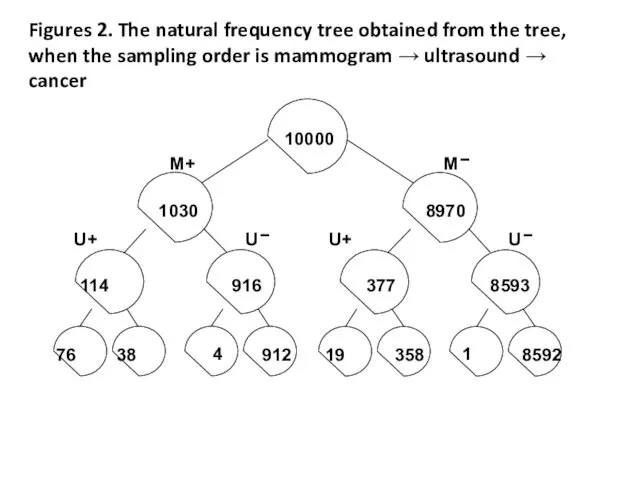
Figures 2. The natural frequency tree obtained from the tree,
Figures 2. The natural frequency tree obtained from the tree,
Organizing the tree in the diagnostic direction produces a much more
Organizing the tree in the diagnostic direction produces a much more
System analysis and decision making
Second, once we have placed a
System analysis and decision making
Second, once we have placed a
That is, the probability comparing the leaves of Figures 1 and
That is, the probability comparing the leaves of Figures 1 and
System analysis and decision making
Knowledge tends to be organised causally,
System analysis and decision making
Knowledge tends to be organised causally,
System analysis and decision making
However, ecologically situated agents tend to
System analysis and decision making
However, ecologically situated agents tend to
System analysis and decision making
Now, consider another version of the
System analysis and decision making
Now, consider another version of the
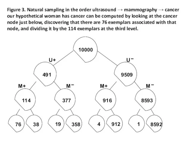
Figure 3. Natural sampling in the order ultrasound → mammography
Figure 3. Natural sampling in the order ultrasound → mammography
System analysis and decision making
FAST AND FRUGAL TREES
A tree may
System analysis and decision making
FAST AND FRUGAL TREES
A tree may
System analysis and decision making
An important convention has to be
System analysis and decision making
An important convention has to be
System analysis and decision making
Definition
A fast and frugal binary decision
System analysis and decision making
Definition
A fast and frugal binary decision
System analysis and decision making
We begin by recalling that according
System analysis and decision making
We begin by recalling that according
System analysis and decision making
Since this ordering is similar to
System analysis and decision making
Since this ordering is similar to
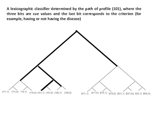
A lexicographic classifier determined by the path of profile (101),
A lexicographic classifier determined by the path of profile (101),
System analysis and decision making
A “lexicographic decision rule” makes one
System analysis and decision making
A “lexicographic decision rule” makes one
Constructing Fast and Frugal Decision Trees
Situation: A man is
Constructing Fast and Frugal Decision Trees
Situation: A man is
Green and Mehr (1997) analyzed the problem of finding a
Green and Mehr (1997) analyzed the problem of finding a
System analysis and decision making
Although Green and Mehr (1997) succeeded
System analysis and decision making
Although Green and Mehr (1997) succeeded
System analysis and decision making
In order to construct a fast
System analysis and decision making
In order to construct a fast
System analysis and decision making
In conceptual analogy to Bayes models,
System analysis and decision making
In conceptual analogy to Bayes models,
System analysis and decision making
The Shape of Trees
There are four
System analysis and decision making
The Shape of Trees
There are four
System analysis and decision making
System analysis and decision making
System analysis and decision making
Trees of type 1 and 4
System analysis and decision making
Trees of type 1 and 4
System analysis and decision making
Trees of types 2 and 3
System analysis and decision making
Trees of types 2 and 3
System analysis and decision making
Cue interactions go beyond the bivariate contingencies
System analysis and decision making
Cue interactions go beyond the bivariate contingencies
Meehl’s paradox in the binary case
Meehl’s paradox in the binary case
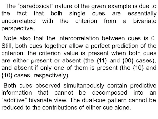
The “paradoxical” nature of the given example is due
The “paradoxical” nature of the given example is due
System analysis and decision making
Correlations between cue 1 and the
System analysis and decision making
Correlations between cue 1 and the
System analysis and decision making
Another way to put it is
System analysis and decision making
Another way to put it is
System analysis and decision making
Representation of Meehl’s paradox in a
System analysis and decision making
Representation of Meehl’s paradox in a
System analysis and decision making
Simple trees bet on a certain
System analysis and decision making
Simple trees bet on a certain
System analysis and decision making
From a statistical point of view,
System analysis and decision making
From a statistical point of view,
System analysis and decision making
For instance, even for large epidemiological
System analysis and decision making
For instance, even for large epidemiological
System analysis and decision making
The fact that cue interactions can
System analysis and decision making
The fact that cue interactions can
 Main features of CSS
 Компьютерные сети. Интернет
 Документ РосБизнесКонсалтинг. Использованы шаблоны MICROSOFT Corp. ©
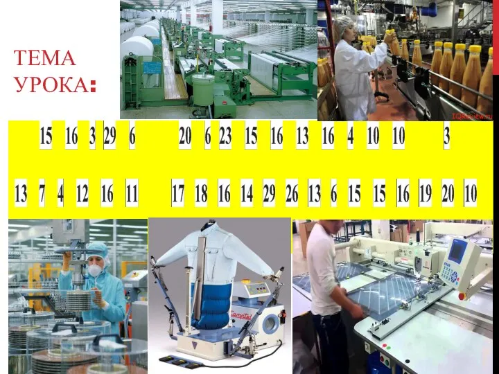 Автоматизация в легкой промышленности
 Задание на 10 марта 6 класс
 Паттерн Репозиторий
 Кодирование информации. 5 класс
 Объекты ядра Windows
 Основы построения инфокоммуникационных систем и сетей
 Информационное моделирование
 Разработка программного модуля проверки на столкновения в Navisworks Simulate
 Табличный процессор MS Excel 2007: формулы и функции
 Бесплатный онлайн квест по автоматизации бизнеса в соцсетях
 Методы системного анализа. Лекция 2
 Общественное объединение родителей Бумеранг добра
 WORD-тын графикалык мумкіндіктері
 Язык HTML. Начальные сведения
 Настройка пользовательского интерфейса Microsoft Word. Лекция 7
 Технология программирования. Функции и структуры
 Тезаурус курса Математика и информатика и ОИКТ
 Объектно-ориентированное программирование
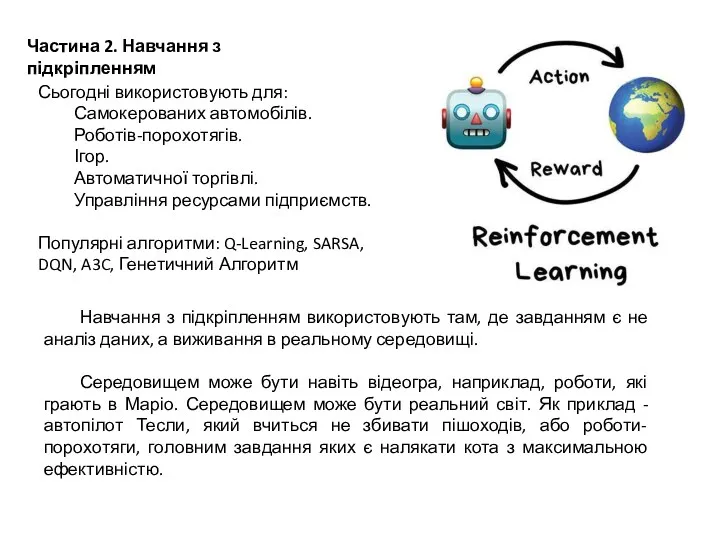 Машинне навчання. Навчання з підкріпленням (частина 2)
 Знакомство с ТРИК Студией
 Пользовательский интерфейс
 MAX mobile - users.pdf
 SQL Server
 Информационные технологии в работе ДОУ
 Телеграмм-бот по игре Dota