- Correlation and Regression

Содержание
- 2. Correlation Correlation A relationship between two variables. The data can be represented by ordered pairs (x,
- 3. Types of Correlation Negative Linear Correlation No Correlation Positive Linear Correlation Nonlinear Correlation As x increases,
- 4. Example: Constructing a Scatter Plot A marketing manager conducted a study to determine whether there is
- 5. Constructing a Scatter Plot Using Technology Enter the x-values into list L1 and the y-values into
- 6. Correlation Coefficient Correlation coefficient A measure of the strength and the direction of a linear relationship
- 7. Linear Correlation Strong negative correlation Weak positive correlation Strong positive correlation Nonlinear Correlation r = −0.91
- 8. Calculating a Correlation Coefficient Find the sum of the x-values. Find the sum of the y-values.
- 9. Example: Finding the Correlation Coefficient Calculate the correlation coefficient for the advertising expenditures and company sales
- 10. Finding the Correlation Coefficient Example Continued… Σx = 15.8 Σy = 1634 Σxy = 3289.8 Σx2
- 11. Using a Table to Test a Population Correlation Coefficient ρ Once the sample correlation coefficient r
- 12. Hypothesis Testing for a Population Correlation Coefficient ρ A hypothesis test (one or two tailed) can
- 13. Using the t-Test for ρ State the null and alternative hypothesis. Specify the level of significance.
- 14. Example: t-Test for a Correlation Coefficient For the advertising data, we previously calculated r ≈ 0.9129.
- 15. Correlation and Causation The fact that two variables are strongly correlated does not in itself imply
- 16. 9.2 Objectives Find the equation of a regression line Predict y-values using a regression equation Larson/Farber
- 17. Residuals & Equation of Line of Regression Residual The difference between the observed y-value and the
- 18. Finding Equation for Line of Regression Larson/Farber 4th ed. 540 294.4 440 624 252 294.4 372
- 19. Solution: Finding the Equation of a Regression Line To sketch the regression line, use any two
- 20. Example: Predicting y-Values Using Regression Equations The regression equation for the advertising expenses (in thousands of
- 21. 9.3 Measures of Regression and Prediction Intervals (Objectives) Interpret the three types of variation about a
- 22. Total variation = The sum of the squares of the differences between the y-value of each
- 23. The Standard Error of Estimate Standard error of estimate The standard deviation (se )of the observed
- 25. Скачать презентацию
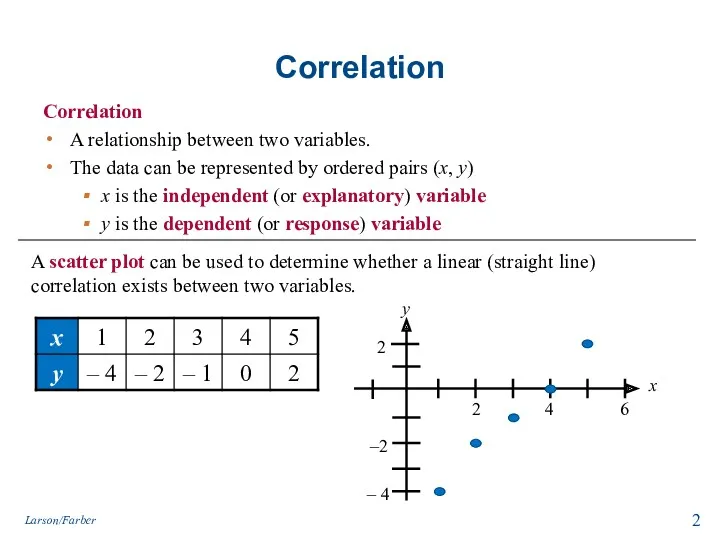
Correlation
Correlation
A relationship between two variables.
The data can be represented
Correlation
Correlation
A relationship between two variables.
The data can be represented
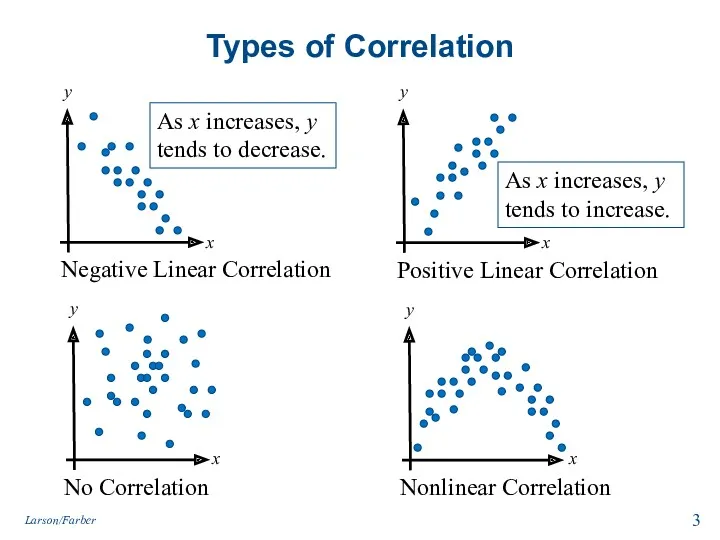
Types of Correlation
Negative Linear Correlation
No Correlation
Positive Linear Correlation
Nonlinear Correlation
As x increases,
Types of Correlation
Negative Linear Correlation
No Correlation
Positive Linear Correlation
Nonlinear Correlation
As x increases,
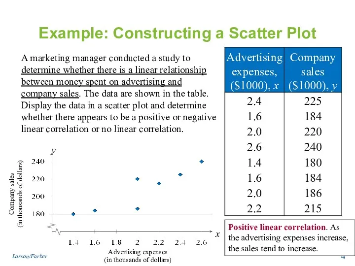
Example: Constructing a Scatter Plot
A marketing manager conducted a study to
Example: Constructing a Scatter Plot
A marketing manager conducted a study to
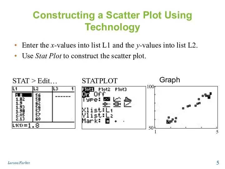
Constructing a Scatter Plot Using Technology
Enter the x-values into list L1
Constructing a Scatter Plot Using Technology
Enter the x-values into list L1
Correlation Coefficient
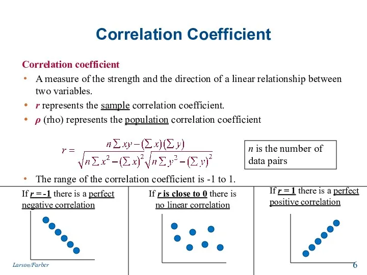
Correlation coefficient
A measure of the strength and the direction of
Correlation Coefficient
Correlation coefficient
A measure of the strength and the direction of
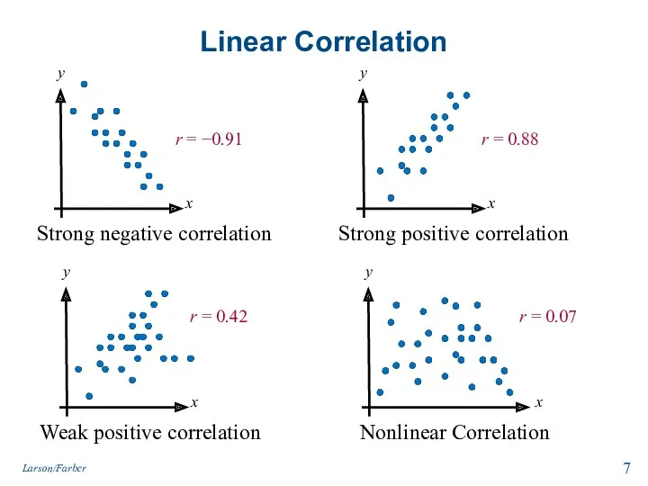
Linear Correlation
Strong negative correlation
Weak positive correlation
Strong positive correlation
Nonlinear Correlation
r = −0.91
r
Linear Correlation
Strong negative correlation
Weak positive correlation
Strong positive correlation
Nonlinear Correlation
r = −0.91
r
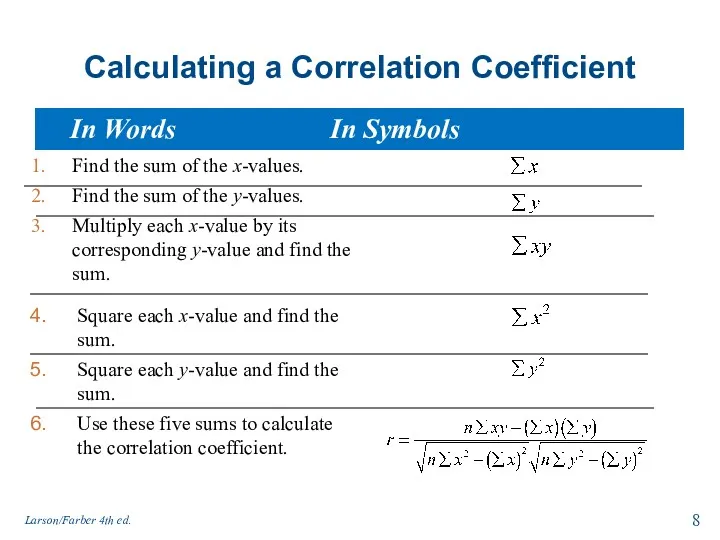
Calculating a Correlation Coefficient
Find the sum of the x-values.
Find the sum
Calculating a Correlation Coefficient
Find the sum of the x-values.
Find the sum
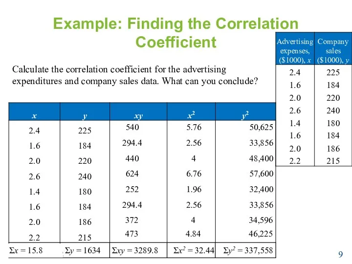
Example: Finding the Correlation Coefficient
Calculate the correlation coefficient for the advertising
Example: Finding the Correlation Coefficient
Calculate the correlation coefficient for the advertising
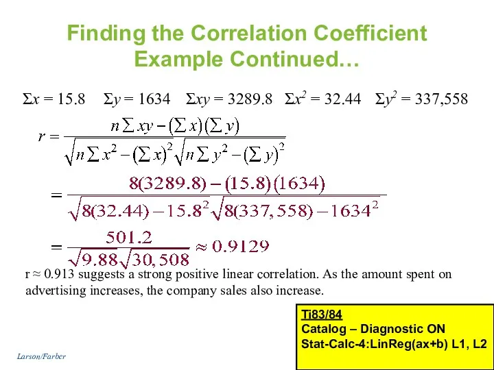
Finding the Correlation Coefficient
Example Continued…
Σx = 15.8
Σy = 1634
Σxy = 3289.8
Σx2
Finding the Correlation Coefficient
Example Continued…
Σx = 15.8
Σy = 1634
Σxy = 3289.8
Σx2
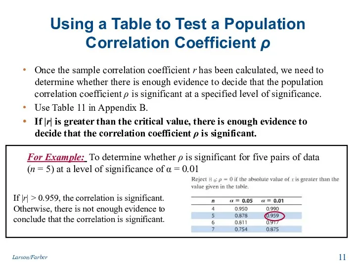
Using a Table to Test a Population Correlation Coefficient ρ
Once the
Using a Table to Test a Population Correlation Coefficient ρ
Once the
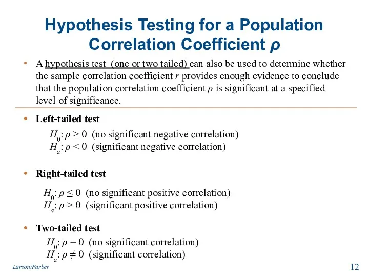
Hypothesis Testing for a Population Correlation Coefficient ρ
A hypothesis test (one
Hypothesis Testing for a Population Correlation Coefficient ρ
A hypothesis test (one
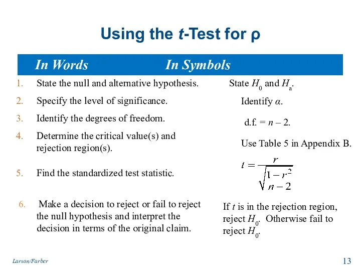
Using the t-Test for ρ
State the null and alternative hypothesis.
Specify the
Using the t-Test for ρ
State the null and alternative hypothesis.
Specify the
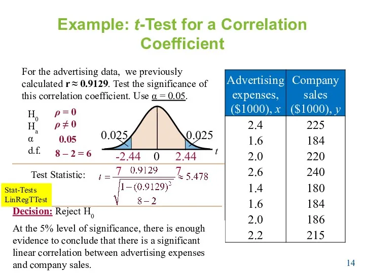
Example: t-Test for a Correlation Coefficient
For the advertising data, we previously
Example: t-Test for a Correlation Coefficient
For the advertising data, we previously

Correlation and Causation
The fact that two variables are strongly correlated does
Correlation and Causation
The fact that two variables are strongly correlated does
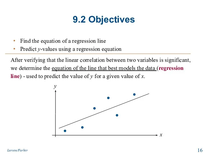
9.2 Objectives
Find the equation of a regression line
Predict y-values using a
9.2 Objectives
Find the equation of a regression line
Predict y-values using a
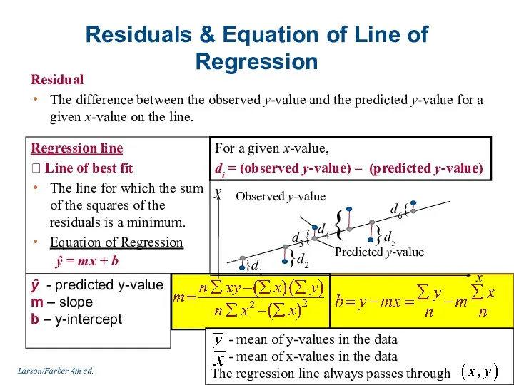
Residuals & Equation of Line of Regression
Residual
The difference between the observed
Residuals & Equation of Line of Regression
Residual
The difference between the observed
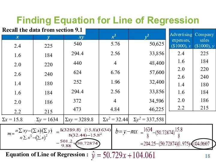
Finding Equation for Line of Regression
Larson/Farber 4th ed.
540
294.4
440
624
252
294.4
372
473
5.76
2.56
4
6.76
1.96
2.56
4
4.84
50,625
33,856
48,400
57,600
32,400
33,856
34,596
46,225
Σx = 15.8
Σy =
Finding Equation for Line of Regression
Larson/Farber 4th ed.
540
294.4
440
624
252
294.4
372
473
5.76
2.56
4
6.76
1.96
2.56
4
4.84
50,625
33,856
48,400
57,600
32,400
33,856
34,596
46,225
Σx = 15.8
Σy =
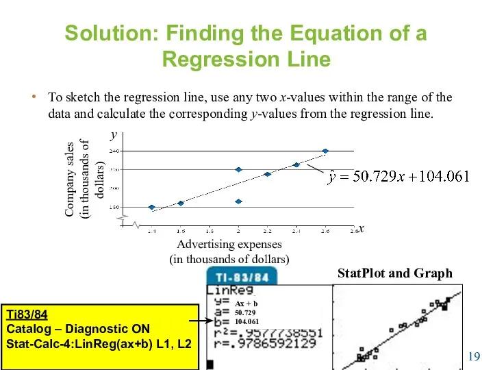
Solution: Finding the Equation of a Regression Line
To sketch the regression
Solution: Finding the Equation of a Regression Line
To sketch the regression
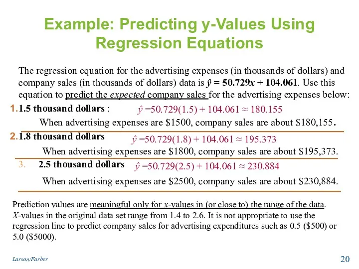
Example: Predicting y-Values Using Regression Equations
The regression equation for the advertising
Example: Predicting y-Values Using Regression Equations
The regression equation for the advertising
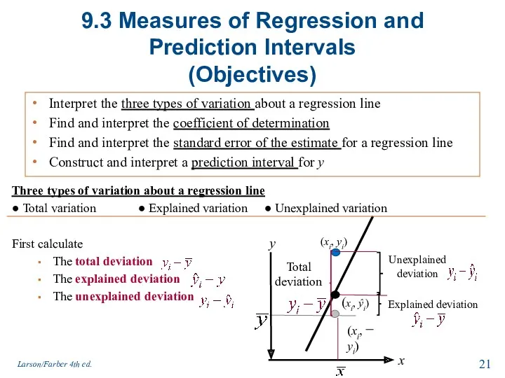
9.3 Measures of Regression and Prediction Intervals
(Objectives)
Interpret the three types of
9.3 Measures of Regression and Prediction Intervals
(Objectives)
Interpret the three types of
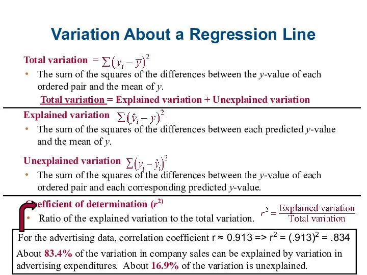
Total variation =
The sum of the squares of the differences
Total variation =
The sum of the squares of the differences
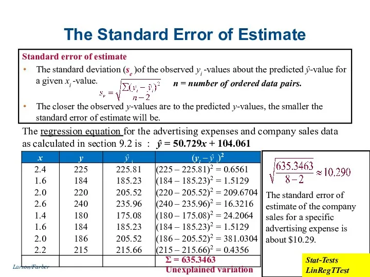
The Standard Error of Estimate
Standard error of estimate
The standard deviation (se
The Standard Error of Estimate
Standard error of estimate
The standard deviation (se
 Натуральные числа. Обозначение натуральных чисел
 Геометрический смысл производной. Задачи типа В8 в ЕГЭ
 Презентация Деление с остатком
 Доли. Обыкновенные дроби. 5 класс
 Единицы времени УМК Гармония 4 класс УМК Гармония
 Конструирование системы задач по теме Линейная функция
 ОТКРЫТЫЙ УРОК ПО МАТЕМАТИКЕ В 4 А КЛАССЕ ПО ТЕМЕ: АРИФМЕТИЧЕСКИЕ ДЕЙСТВИЯ НАД ЧИСЛАМИ
 Решение систем линейных уравнений с двумя переменными
 Знаходження числа за його відсотком
 Франсуа Виет
 Дерево возможных вариантов
 Математика. Основные разделы теста. 1 семестр
 Круги Эйлера в решении задач
 Одночлены и многочлены
 Закон больших чисел
 Единицы времени УМК Гармония 4 класс УМК Гармония
 Задачи на увеличение и уменьшение на несколько единиц
 Состав чисел второго десятка с переходом через десяток
 Многоугольники. Четырехугольники
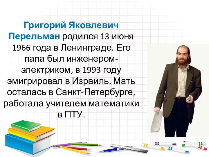 Григорий Яковлевич Перельман
 Решение задач. 1 класс
 Действия с рациональными числами
 Умножение десятичных дробей
 Что такое топология. Лист Мёбиуса
 Комплексные числа. Типовой вариант самостоятельной работы
 Сложение натуральных чисел и его свойства
 Задания типа С5
 Период радиоактивного распада. Решение задач. Интегрированный урок физика+математика 11 класс