- Exploring Assumptions Normality and Homogeneity of Variance

Содержание
- 2. Outliers Impact
- 3. Assumptions Parametric tests based on the normal distribution assume: Additivity and linearity Normality something or other
- 4. Additivity and Linearity The outcome variable is, in reality, linearly related to any predictors. If you
- 5. Normality Something or Other The normal distribution is relevant to: Parameters Confidence intervals around a parameter
- 6. When does the Assumption of Normality Matter? In small samples – The central limit theorem allows
- 7. Spotting Normality
- 8. The P-P Plot
- 9. Assessing Skew and Kurtosis
- 11. Homoscedasticity/ Homogeneity of Variance When testing several groups of participants, samples should come from populations with
- 12. Assessing Homoscedasticity/ Homogeneity of Variance Graphs (see lectures on regression) Levene’s Tests Tests if variances in
- 14. Homogeneity of Variance
- 15. Independence The errors in your model should not be related to each other. If this assumption
- 16. Reducing Bias Trim the data: Delete a certain amount of scores from the extremes. Windsorizing: Substitute
- 17. Trimming the Data
- 18. Robust Methods
- 19. Transforming Data
- 20. Log Transformation
- 21. Square Root Transformation
- 22. Reciprocal Transformation
- 23. But …
- 25. Скачать презентацию
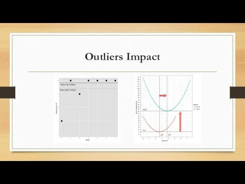
Outliers Impact
Outliers Impact
Assumptions
Parametric tests based on the normal distribution assume:
Additivity and linearity
Assumptions
Parametric tests based on the normal distribution assume:
Additivity and linearity
Additivity and Linearity
The outcome variable is, in reality, linearly related to
Additivity and Linearity
The outcome variable is, in reality, linearly related to
Normality Something or Other
The normal distribution is relevant to:
Parameters
Normality Something or Other
The normal distribution is relevant to:
Parameters
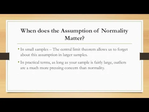
When does the Assumption of Normality Matter?
In small samples – The
When does the Assumption of Normality Matter?
In small samples – The
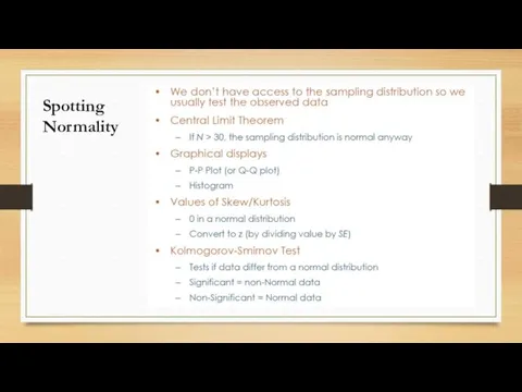
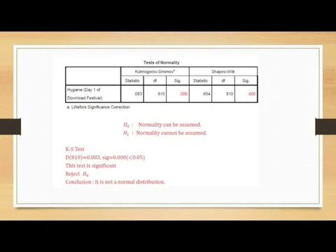
Spotting
Normality
Spotting
Normality
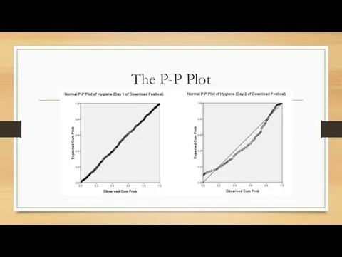
The P-P Plot
The P-P Plot
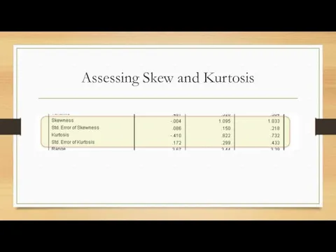
Assessing Skew and Kurtosis
Assessing Skew and Kurtosis
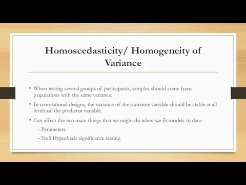
Homoscedasticity/ Homogeneity of Variance
When testing several groups of participants, samples
Homoscedasticity/ Homogeneity of Variance
When testing several groups of participants, samples
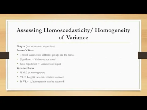
Assessing Homoscedasticity/ Homogeneity of Variance
Graphs (see lectures on regression)
Levene’s
Assessing Homoscedasticity/ Homogeneity of Variance
Graphs (see lectures on regression)
Levene’s
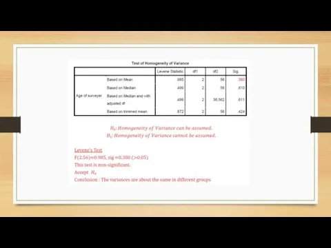
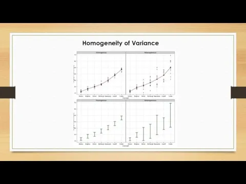
Homogeneity of Variance
Homogeneity of Variance
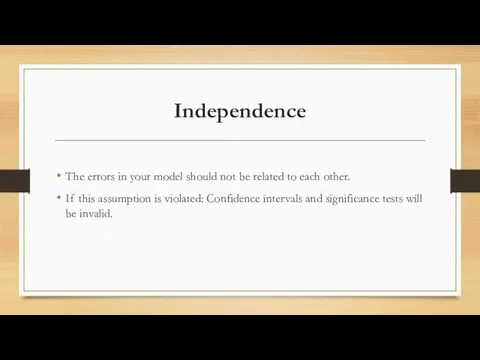
Independence
The errors in your model should not be related to
Independence
The errors in your model should not be related to
Reducing Bias
Trim the data: Delete a certain amount of scores from
Reducing Bias
Trim the data: Delete a certain amount of scores from
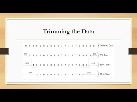
Trimming the Data
Trimming the Data
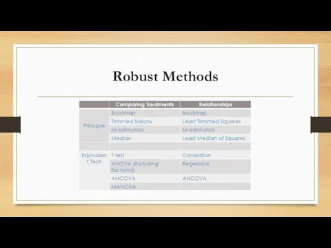
Robust Methods
Robust Methods
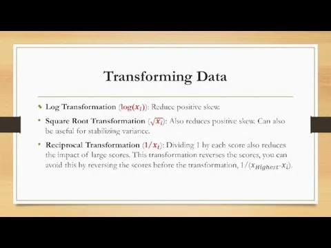
Transforming Data
Transforming Data
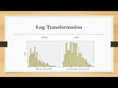
Log Transformation
Log Transformation
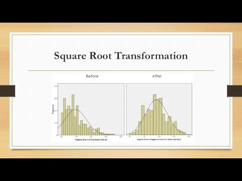
Square Root Transformation
Square Root Transformation
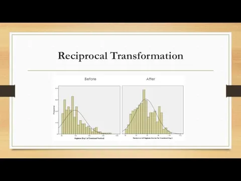
Reciprocal Transformation
Reciprocal Transformation
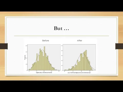
But …
But …
 Определители второго и третьего порядка
 Прямоугольные треугольники и их свойства
 Устные приемы умножения и деления чисел от 1 до 1000; 3 класс. Технологический приём Универсальный тренажёр
 Приём вычитания вида 15 -
 Игры со спичками
 Математика .Презентация Устный счёт.
 Деление с остатком
 Interval Discrete Equation as a Model of Soil and Groundwater Contamination by Nitrogen
 Понятие о доказательной медицине. Случайное событие. Определение вероятности. Лекция 2
 Линейное уравнение с двумя переменными, его график, примеры решения уравнений в целых числах
 Умножение одночленов
 Грецькі вчені-математики
 Диференціальне числення. Похідна функції (лекція 1.2)
 Уравнения и неравенства. Упражнение 2
 Личностно ориентированные технологии на уроках математики
 Задачи на построение сечений тетраэдра и параллелепипеда
 Презентация Прямоугольник, квадрат
 волшебная полянка 1
 Моя страничка на proshkolu.ru
 Передбачення результату виконання алгоритму
 Linear Regression and Correlation Analysis
 Презентация по математике для 1 класса УМК Школа России. По теме: Слагаемые. Сумма.
 Теорема Пифагора
 Рациональные уравнения
 Умножение дробей
 Движение:Скорость,время,расстояние.
 Статистические характеристики. Основные статистические характеристики. 7 класс
 Четырехугольники. Геометрия 8 класс