- Linear Regression and Correlation Analysis

Содержание
- 2. Learning Outcomes Outcome 1. Calculate and interpret the correlation between two variables. Outcome 2. Determine whether
- 3. 14.1 Scatter Plots and Correlation Scatter Plot A two-dimensional plot showing the values for the joint
- 4. Two-Variable Relationships
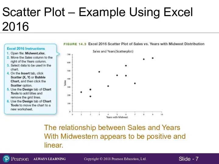
- 5. Scatter Plot – Example Using Excel 2016 The director of marketing for Midwest Distribution Company is
- 6. Scatter Plot – Example Using Excel 2016 Sample Data: Sales and Years With Midwestern
- 7. Scatter Plot – Example Using Excel 2016 The relationship between Sales and Years With Midwestern appears
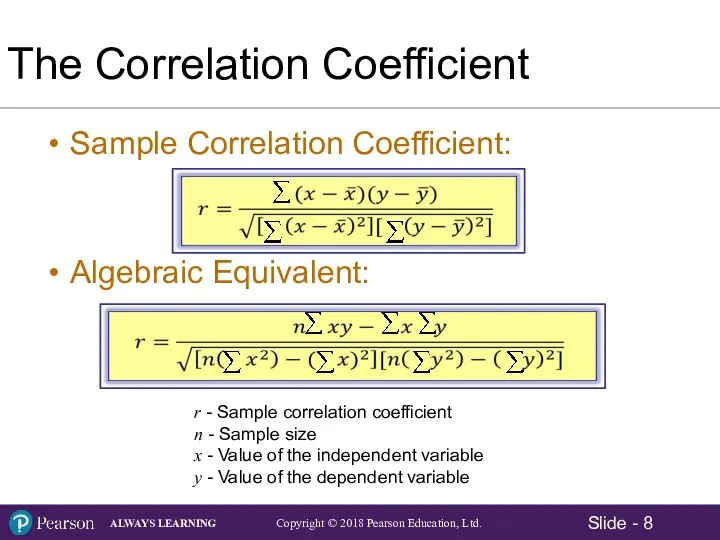
- 8. The Correlation Coefficient Sample Correlation Coefficient: Algebraic Equivalent: r - Sample correlation coefficient n - Sample
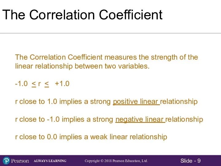
- 9. The Correlation Coefficient The Correlation Coefficient measures the strength of the linear relationship between two variables.
- 10. Correlation between Two Variables
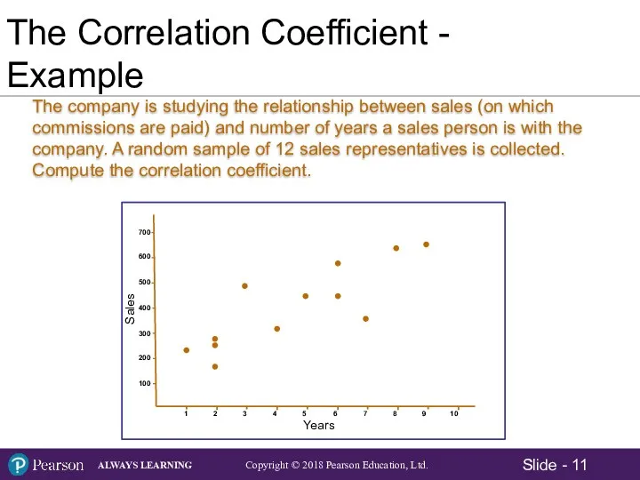
- 11. The Correlation Coefficient - Example The company is studying the relationship between sales (on which commissions
- 12. The Correlation Coefficient – Manual Calculation Example
- 13. 1. Open file: Midwest.xlsx. 2. Select Data > Data Analysis. 3. Select Correlation. 4. Define the
- 14. Significance Test for the Correlation The Null and Alternative Hypotheses: Test Statistic for Correlation: Assumptions: The
- 15. Significance Test for the Correlation - Example Midwestern Example
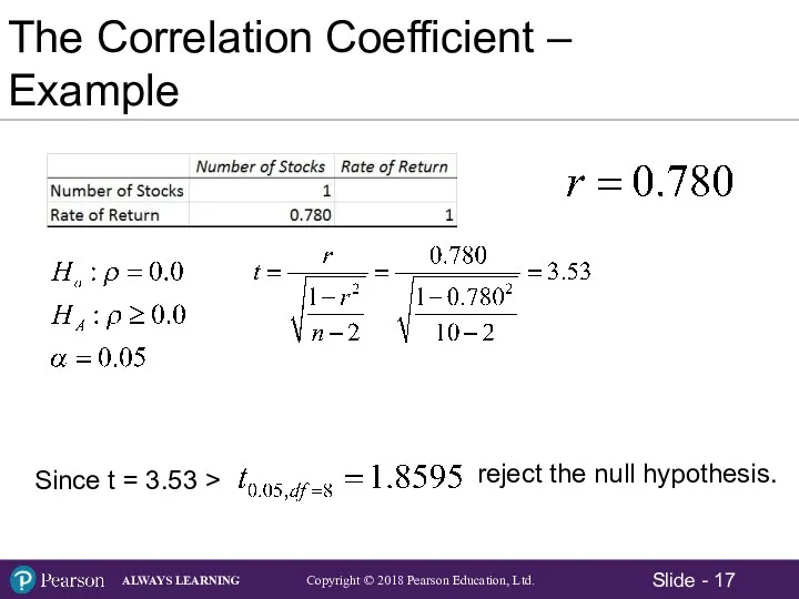
- 16. The Correlation Coefficient – Example A money management company is interested in determining whether there is
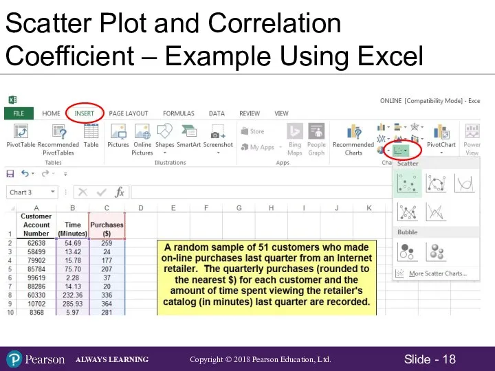
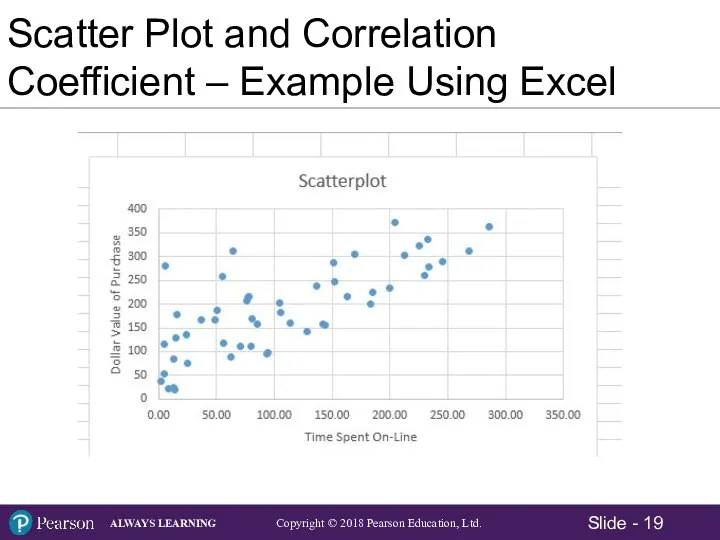
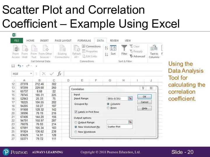
- 19. Scatter Plot and Correlation Coefficient – Example Using Excel
- 20. Scatter Plot and Correlation Coefficient – Example Using Excel Using the Data Analysis Tool for calculating
- 22. Correlation Analysis - Summary Step 1: Specify the population parameter of interest Step 2: Formulate the
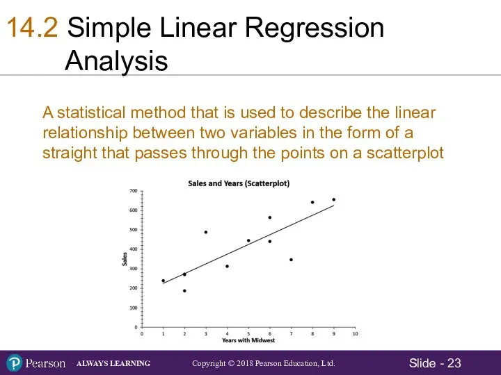
- 23. 14.2 Simple Linear Regression Analysis A statistical method that is used to describe the linear relationship
- 24. Simple Linear Regression Analysis When there are only two variables - a dependent variable, and an
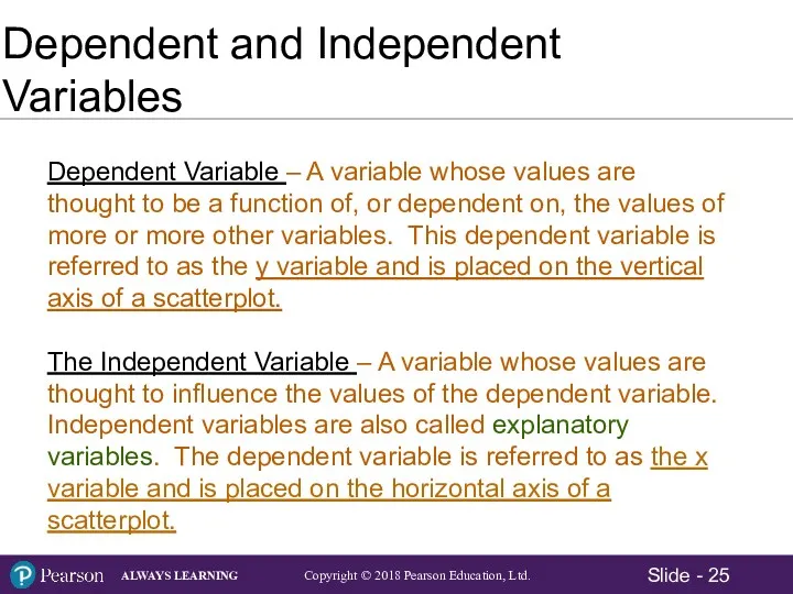
- 25. Dependent and Independent Variables Dependent Variable – A variable whose values are thought to be a
- 26. The Regression Model
- 28. Linear Regression Assumptions – Visual Representation
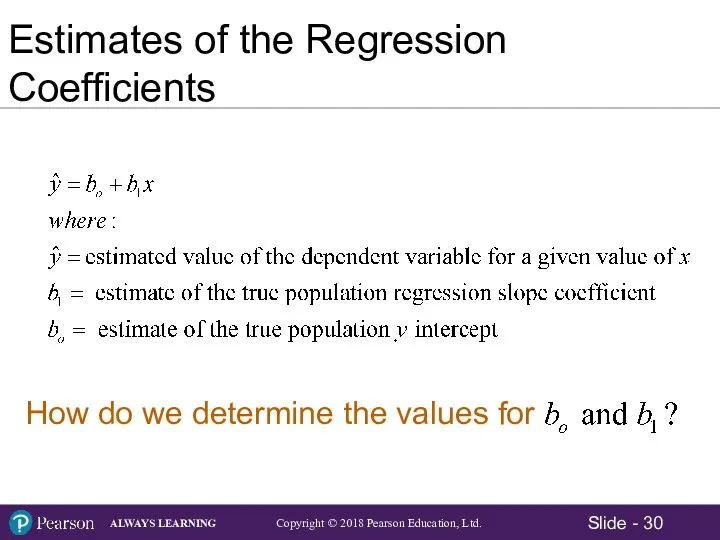
- 29. Meaning of the Regression Coefficients
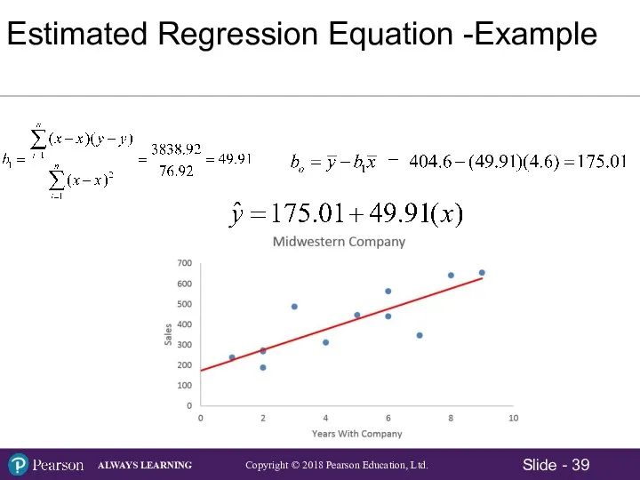
- 31. Regression Line Examples
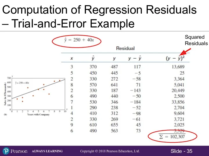
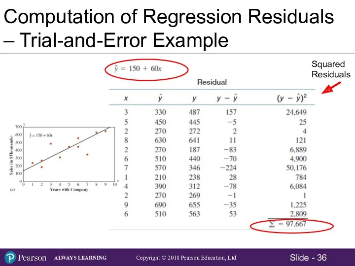
- 32. Computation of Regression Error - Example
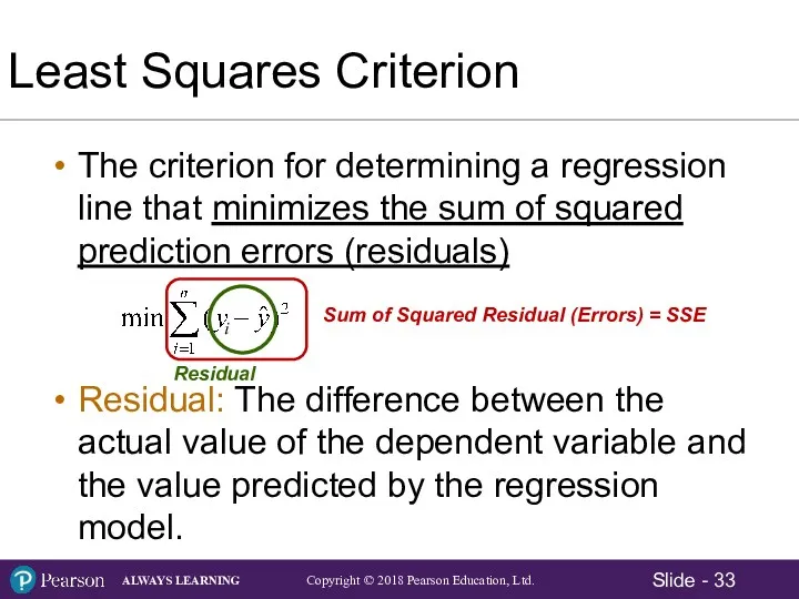
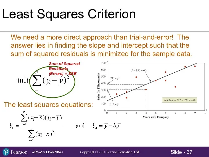
- 33. Least Squares Criterion The criterion for determining a regression line that minimizes the sum of squared
- 34. Sum of Squared Residuals (Errors) =
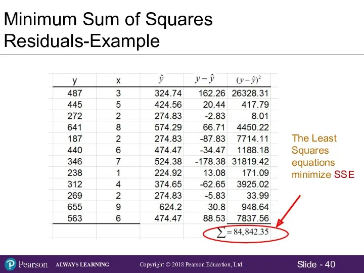
- 37. i i i i Sum of Squared Residuals (Errors) = SSE
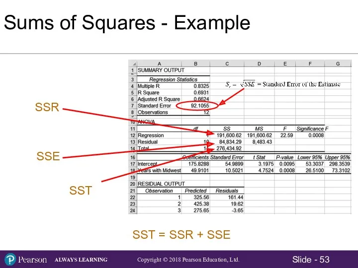
- 41. Excel 2016 Regression Results
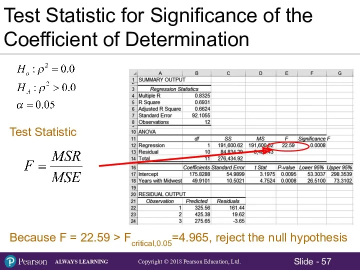
- 42. Test for Significance of the Regression Slope Coefficient
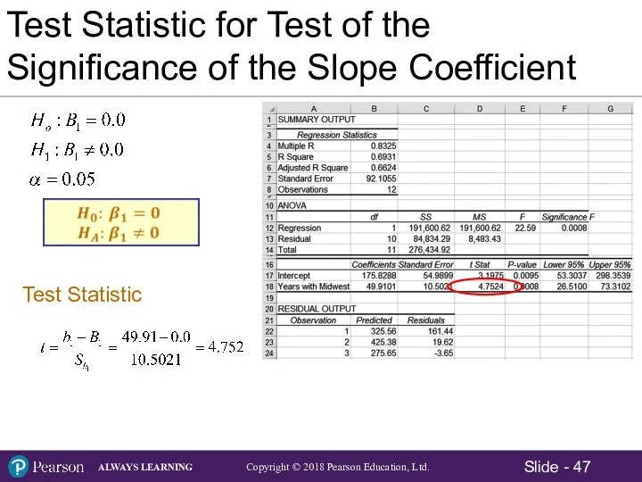
- 43. Test Statistic for Test of the Significance of the Slope Coefficient Hypotheses: Test Statistic: Test Statistic
- 44. Standard Error of the Slope Simple Regression Estimator for the Standard Error of the Slope:
- 45. Standard Error of the Slope Large Standard Error Small Standard Error
- 46. Standard Error of the Slope- Example Sε Sε MSE
- 47. Test Statistic for Test of the Significance of the Slope Coefficient
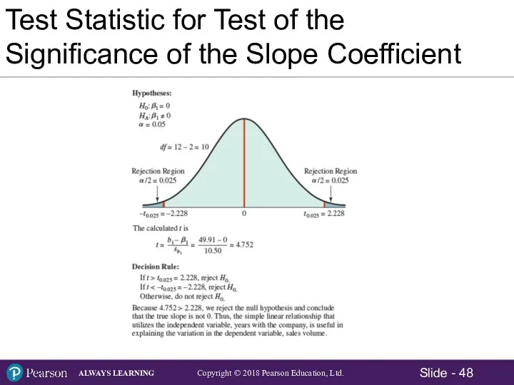
- 48. Test Statistic for Test of the Significance of the Slope Coefficient
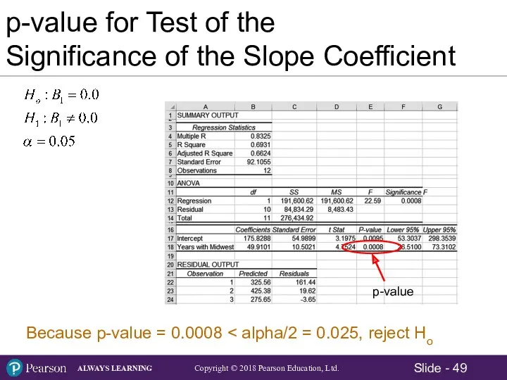
- 49. p-value for Test of the Significance of the Slope Coefficient
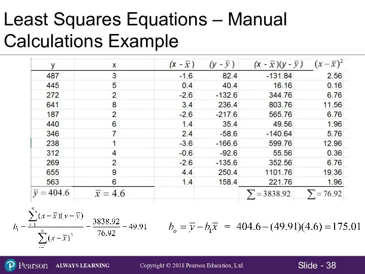
- 50. Review: The Correlation Coefficient – Manual Calculation Example
- 51. Sums of Squares The portion of the total variation in the dependent variable that is explained
- 52. Sums of Squares Total Sum of Squares: Sum of Squares Regression: Sum of Squared Residual (Errors)
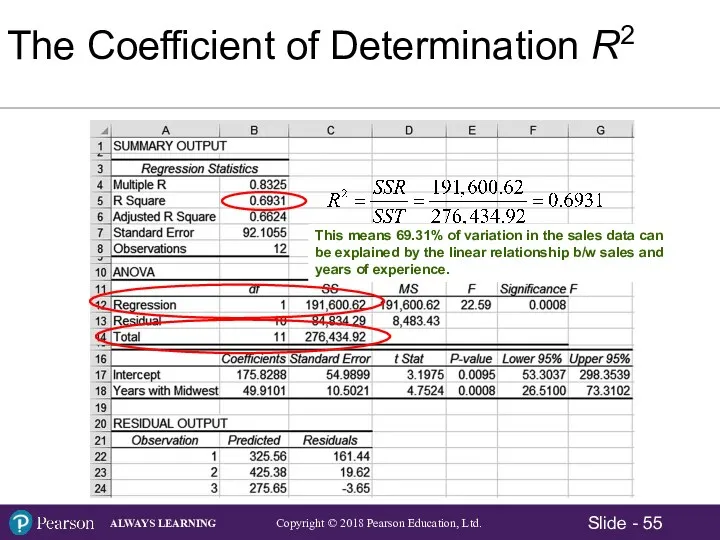
- 54. The Coefficient of Determination R2 The portion of the total variation in the dependent variable that
- 55. This means 69.31% of variation in the sales data can be explained by the linear relationship
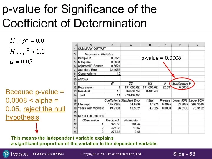
- 58. This means the independent variable explains a significant proportion of the variation in the dependent variable.
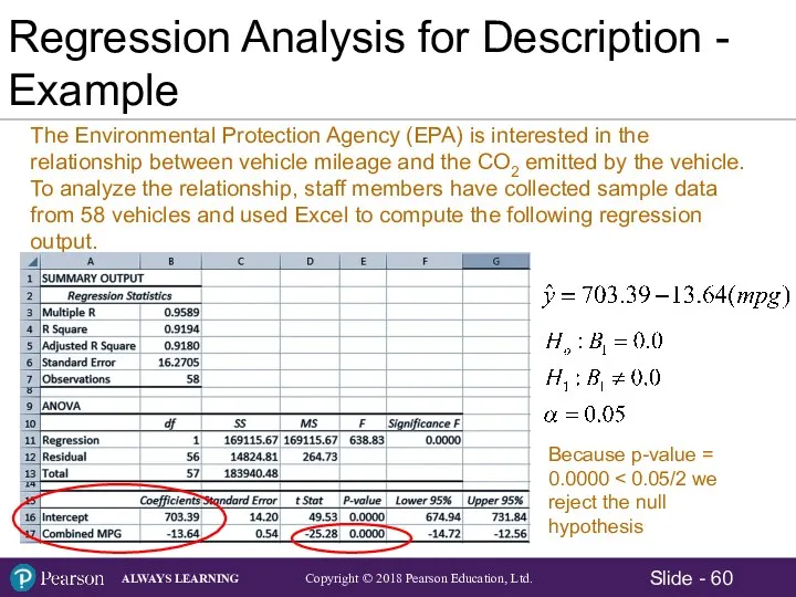
- 59. 14.3 Uses for Regression Analysis Description – When we are primarily interested in analyzing the relationship
- 60. Regression Analysis for Description - Example
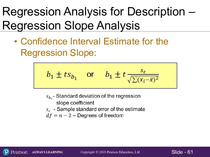
- 61. Regression Analysis for Description – Regression Slope Analysis Confidence Interval Estimate for the Regression Slope:
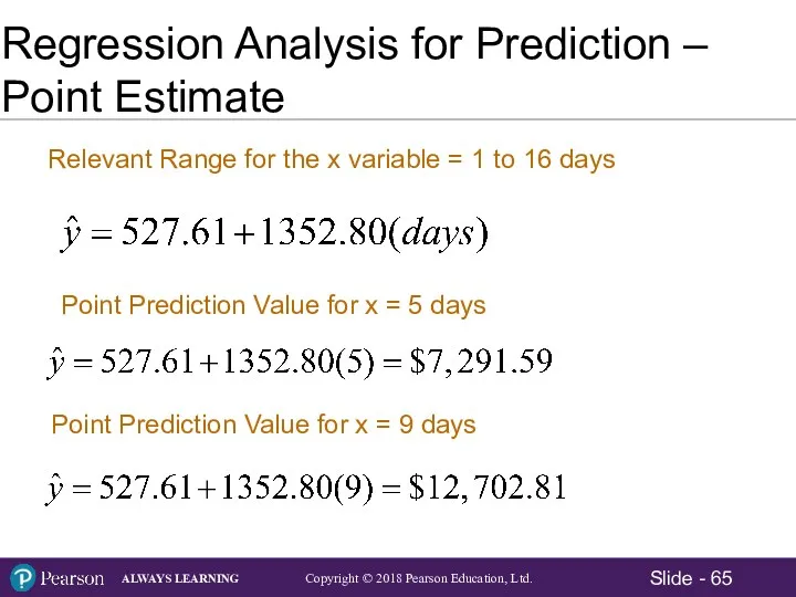
- 65. Regression Analysis for Prediction – Point Estimate Relevant Range for the x variable = 1 to
- 68. Potential Variation in y as xp Moves Farther from
- 69. Confidence and Prediction Intervals
- 71. Скачать презентацию
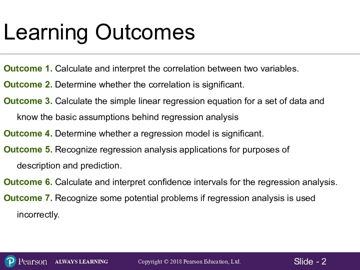
Learning Outcomes
Outcome 1. Calculate and interpret the correlation between two variables.
Outcome
Learning Outcomes
Outcome 1. Calculate and interpret the correlation between two variables.
Outcome
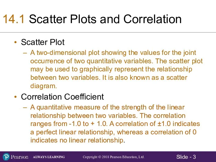
14.1 Scatter Plots and Correlation
Scatter Plot
A two-dimensional plot showing the
14.1 Scatter Plots and Correlation
Scatter Plot
A two-dimensional plot showing the
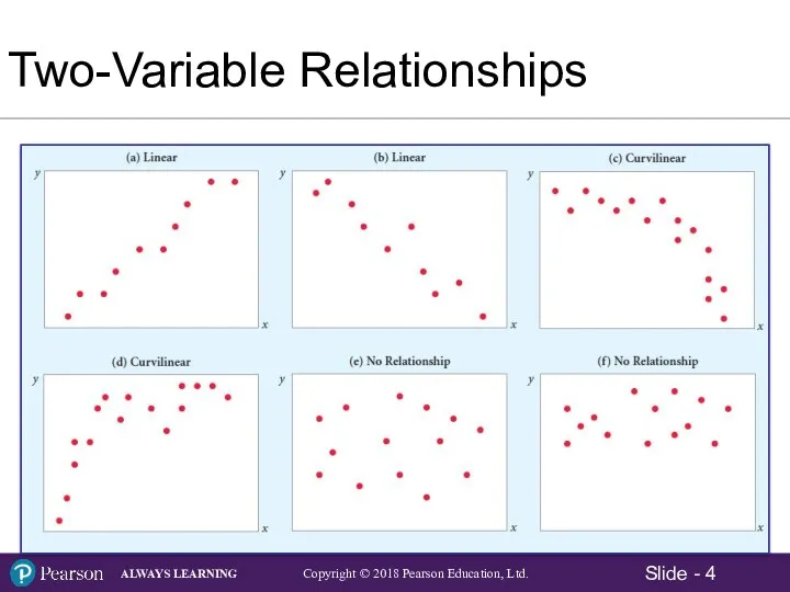
Two-Variable Relationships
Two-Variable Relationships
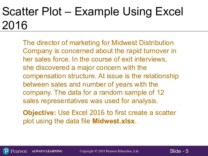
Scatter Plot – Example Using Excel 2016
The director of marketing for
Scatter Plot – Example Using Excel 2016
The director of marketing for

Scatter Plot – Example Using Excel 2016
Sample Data: Sales and Years
Scatter Plot – Example Using Excel 2016
Sample Data: Sales and Years
Scatter Plot – Example Using Excel 2016
The relationship between Sales and
Scatter Plot – Example Using Excel 2016
The relationship between Sales and
The Correlation Coefficient
Sample Correlation Coefficient:
Algebraic Equivalent:
r - Sample correlation coefficient
n -
The Correlation Coefficient
Sample Correlation Coefficient:
Algebraic Equivalent:
r - Sample correlation coefficient
n -
The Correlation Coefficient
The Correlation Coefficient measures the strength of the linear
The Correlation Coefficient
The Correlation Coefficient measures the strength of the linear
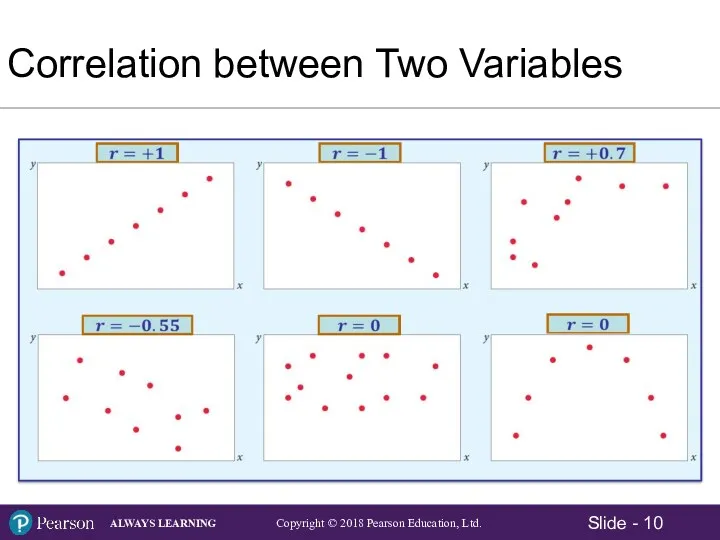
Correlation between Two Variables
Correlation between Two Variables
The Correlation Coefficient - Example
The company is studying the relationship between
The Correlation Coefficient - Example
The company is studying the relationship between

The Correlation Coefficient – Manual Calculation Example
The Correlation Coefficient – Manual Calculation Example
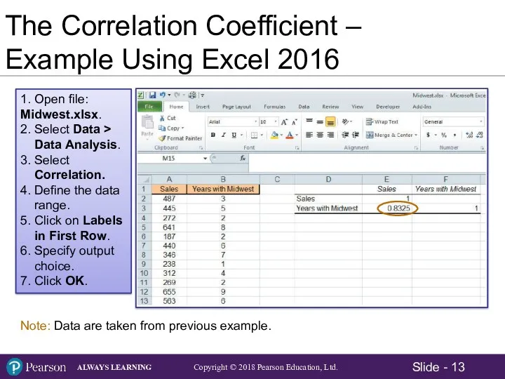
1. Open file: Midwest.xlsx.
2. Select Data > Data Analysis.
3. Select Correlation.
4.
1. Open file: Midwest.xlsx. 2. Select Data > Data Analysis. 3. Select Correlation. 4.
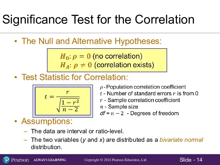
Significance Test for the Correlation
The Null and Alternative Hypotheses:
Test Statistic for
Significance Test for the Correlation
The Null and Alternative Hypotheses:
Test Statistic for
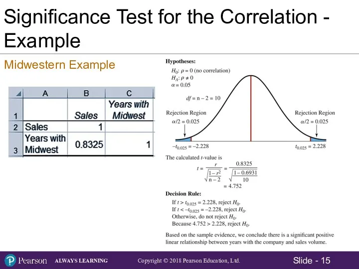
Significance Test for the Correlation - Example
Midwestern Example
Significance Test for the Correlation - Example
Midwestern Example
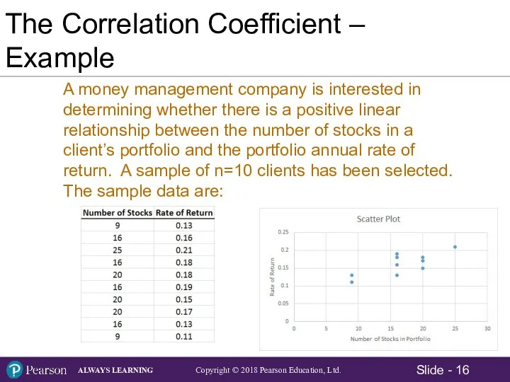
The Correlation Coefficient – Example
A money management company is interested in
The Correlation Coefficient – Example
A money management company is interested in
Scatter Plot and Correlation Coefficient – Example Using Excel
Scatter Plot and Correlation Coefficient – Example Using Excel
Scatter Plot and Correlation Coefficient – Example Using Excel
Using the Data
Scatter Plot and Correlation Coefficient – Example Using Excel
Using the Data

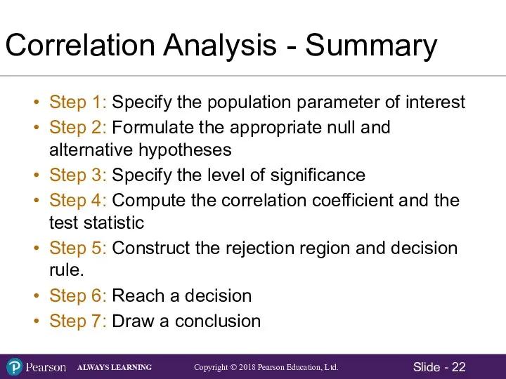
Correlation Analysis - Summary
Step 1: Specify the population parameter of interest
Step
Correlation Analysis - Summary
Step 1: Specify the population parameter of interest
Step
14.2 Simple Linear Regression Analysis
A statistical method that is used to
14.2 Simple Linear Regression Analysis
A statistical method that is used to
Simple Linear Regression Analysis
When there are only two variables - a
Simple Linear Regression Analysis
When there are only two variables - a
Dependent and Independent Variables
Dependent Variable – A variable whose values are
Dependent and Independent Variables
Dependent Variable – A variable whose values are
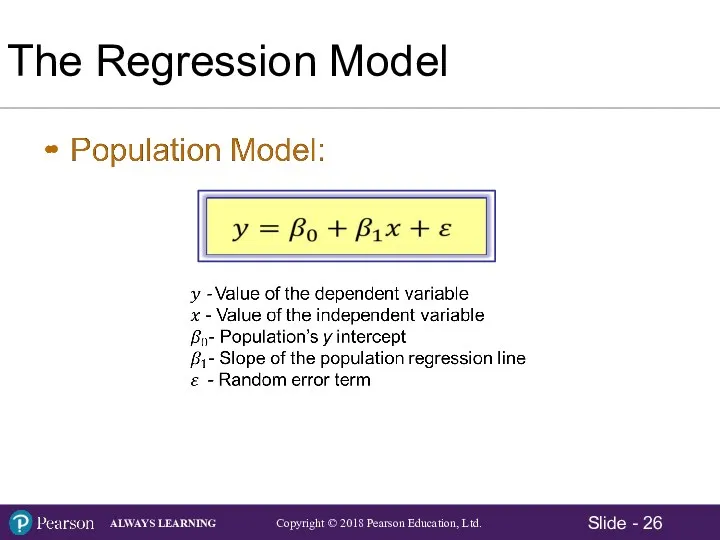
The Regression Model
The Regression Model
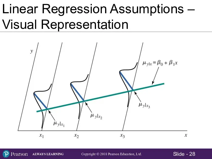
Linear Regression Assumptions – Visual Representation
Linear Regression Assumptions – Visual Representation

Meaning of the Regression Coefficients
Meaning of the Regression Coefficients
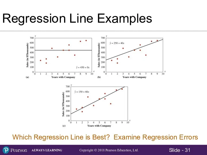
Regression Line Examples
Regression Line Examples
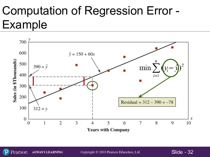
Computation of Regression Error - Example
Computation of Regression Error - Example
Least Squares Criterion
The criterion for determining a regression line that minimizes
Least Squares Criterion
The criterion for determining a regression line that minimizes
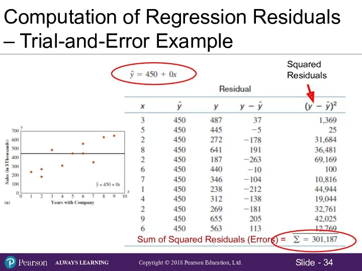
Sum of Squared Residuals (Errors) =
Sum of Squared Residuals (Errors) =
i
i
i
i
Sum of Squared Residuals (Errors) = SSE
i
i
i
i
Sum of Squared Residuals (Errors) = SSE
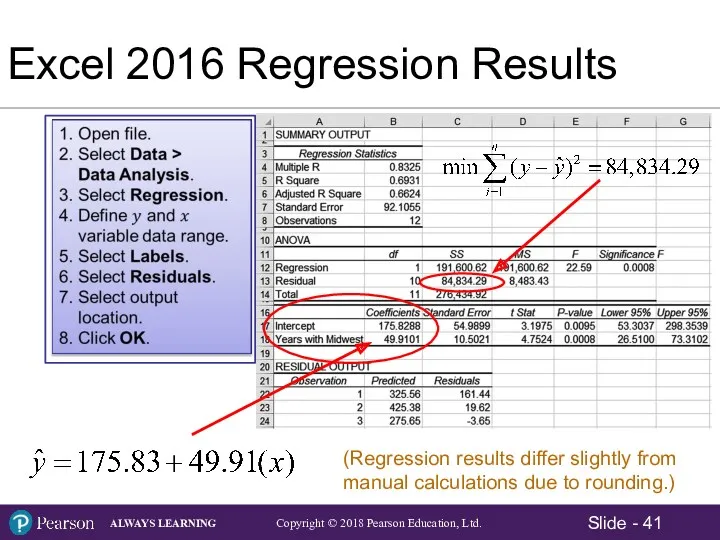
Excel 2016 Regression Results
Excel 2016 Regression Results
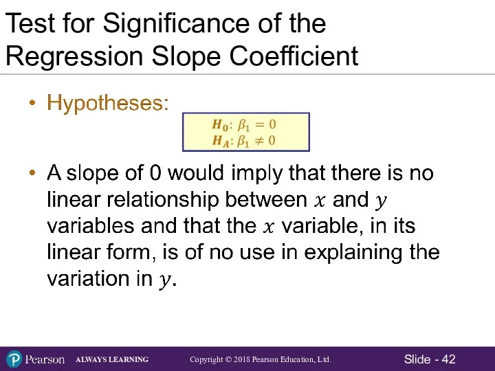
Test for Significance of the Regression Slope Coefficient
Test for Significance of the Regression Slope Coefficient
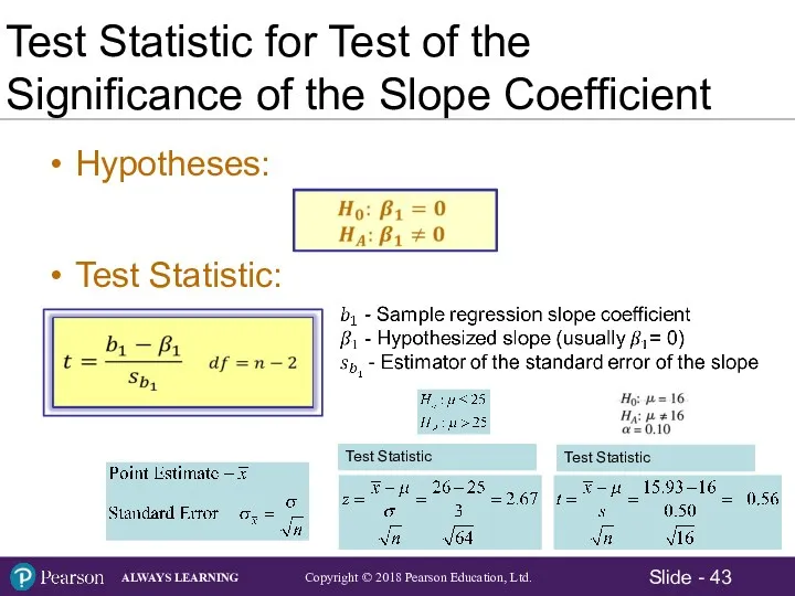
Test Statistic for Test of the
Significance of the Slope Coefficient
Hypotheses:
Test Statistic:
Test
Test Statistic for Test of the
Significance of the Slope Coefficient
Hypotheses:
Test Statistic:
Test
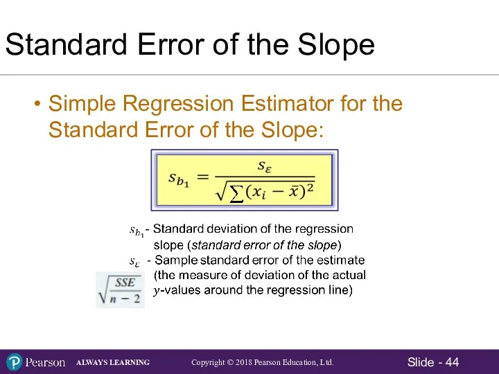
Standard Error of the Slope
Simple Regression Estimator for the Standard Error
Standard Error of the Slope
Simple Regression Estimator for the Standard Error

Standard Error of the Slope
Large Standard Error
Small Standard Error
Standard Error of the Slope
Large Standard Error
Small Standard Error
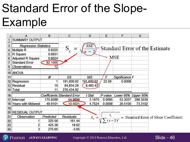
Standard Error of the Slope- Example
Sε
Sε
MSE
Standard Error of the Slope- Example
Sε
Sε
MSE
Test Statistic for Test of the
Significance of the Slope Coefficient
Test Statistic for Test of the
Significance of the Slope Coefficient
Test Statistic for Test of the
Significance of the Slope Coefficient
Test Statistic for Test of the
Significance of the Slope Coefficient
p-value for Test of the
Significance of the Slope Coefficient
p-value for Test of the
Significance of the Slope Coefficient
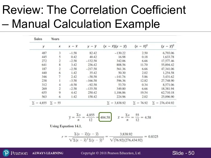
Review: The Correlation Coefficient – Manual Calculation Example
Review: The Correlation Coefficient – Manual Calculation Example
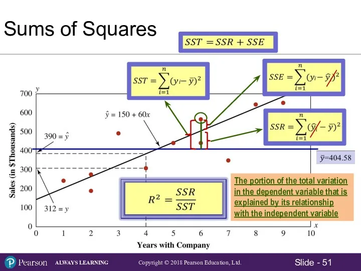
Sums of Squares
The portion of the total variation in the dependent
Sums of Squares
The portion of the total variation in the dependent
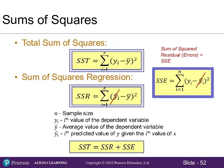
Sums of Squares
Total Sum of Squares:
Sum of Squares Regression:
Sum of
Sums of Squares
Total Sum of Squares:
Sum of Squares Regression:
Sum of
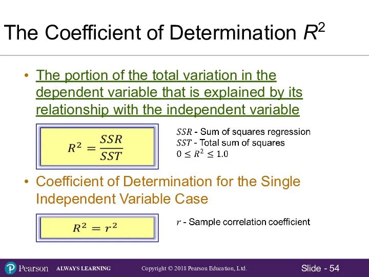
The Coefficient of Determination R2
The portion of the total variation in
The Coefficient of Determination R2
The portion of the total variation in
This means 69.31% of variation in the sales data can be
This means 69.31% of variation in the sales data can be

This means the independent variable explains
a significant proportion of the
This means the independent variable explains
a significant proportion of the
14.3 Uses for Regression Analysis
Description – When we are primarily interested
14.3 Uses for Regression Analysis
Description – When we are primarily interested
Regression Analysis for Description - Example
Regression Analysis for Description - Example
Regression Analysis for Description – Regression Slope Analysis
Confidence Interval Estimate for
Regression Analysis for Description – Regression Slope Analysis
Confidence Interval Estimate for

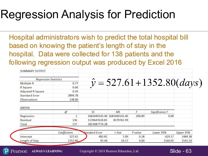
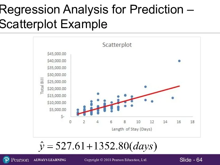
Regression Analysis for Prediction – Point Estimate
Relevant Range for the x
Regression Analysis for Prediction – Point Estimate
Relevant Range for the x

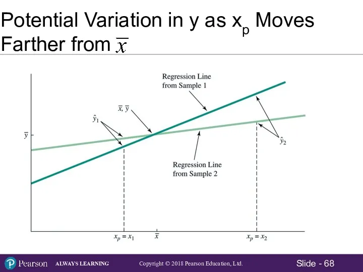
Potential Variation in y as xp Moves Farther from
Potential Variation in y as xp Moves Farther from
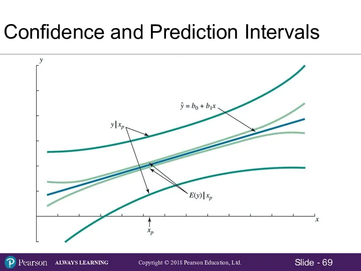
Confidence and Prediction Intervals
Confidence and Prediction Intervals
 Конспект урока и презентация по математике в 4 классе
 Тоғызқұмалақ және математика
 математика. устный счет
 Округление натуральных чисел
 Решение алгебраических и трансцендентных уравнений
 Решение задач по планиметрии
 Классификация треугольников по углам
 Свойства правильных многогранников и их применение
 Алгебра логики
 Урок математики
 Ділення з остачею
 Задачи на деление.
 Дециметр (дм)
 Нахождение дроби от числа
 Урок повторения курса геометрии 7-9
 Свойства действий над числами
 Тест по математике Решение логических задач. 5 класс
 Преподавание алгебры в 7 классе с углубленным изучением математики
 Презентация к уроку математики по программе Перспективная начальная школа
 Билеты по геометрии. Переводной экзамен. 8 класс
 Масса предметов. Килограмм
 Урок математики с презентацией в 1 классе на тему:Закрепление изученного. Проверка знаний
 Среднее арифметическое. Среднее значение величины
 Умножение положительных и отрицательных чисел
 Готовимся к ЕГЭ
 Фрагмент урока. Контрольный тест Числа больше 1000
 Аналіз характеристик КС на основі теорії марківських процесів. (Тема 5)
 Урок математики