- Management Science

Содержание
- 2. Copyright © 2010 Pearson Education, Inc. Publishing as Prentice Hall BA 250 Management Science Management science,
- 3. Text Book Introduction to Management Science Bernard W. Taylor III, 12th Edition, Prentice Hall, New Jersey
- 4. Learning Outcomes The students who succeed in this course; define basic mathematical modeling concepts and techniques
- 5. BA 250 Management Science Copyright © 2010 Pearson Education, Inc. Publishing as Prentice Hall
- 6. EVALUATION SYSTEM PERCENTAGE OF GRADE First Mid-Term Exam 30 Second Mid-Term Exam 30 Final Exam 40
- 7. Copyright © 2010 Pearson Education, Inc. Publishing as Prentice Hall Chapter 1 Topics Examples of Managerial
- 8. Examples of Managerial Problems (Manufacturing) A manufacturer has fixed amounts of different resources such as raw
- 9. Examples of Managerial Problems (Production Scheduling) A manufacturer knows that he must supply a given number
- 10. Examples of Managerial Problems (Transportation) A product is to be shipped in the amounts al, a2,
- 11. Examples of Managerial Problems (Finance: Portfolio Selection Problem) ___________________________________________________________________________ Operations Research © Jan Fábry Maximization of
- 12. Examples of Managerial Problems (Marketing Research) ___________________________________________________________________________ Operations Research © Jan Fábry Evaluating consumer’s reaction to
- 13. Copyright © 2010 Pearson Education, Inc. Publishing as Prentice Hall Figure 1.1 The Management Science Process
- 14. Copyright © 2010 Pearson Education, Inc. Publishing as Prentice Hall Steps in the Management Science Process
- 15. Copyright © 2010 Pearson Education, Inc. Publishing as Prentice Hall Information and Data: Business firm makes
- 16. Copyright © 2010 Pearson Education, Inc. Publishing as Prentice Hall Variables: X = # units to
- 17. Copyright © 2010 Pearson Education, Inc. Publishing as Prentice Hall Example of Model Construction (3 of
- 18. Copyright © 2010 Pearson Education, Inc. Publishing as Prentice Hall Model Building: Break-Even Analysis Used to
- 19. Copyright © 2010 Pearson Education, Inc. Publishing as Prentice Hall Model Components Fixed Cost (cf) -
- 20. Copyright © 2010 Pearson Education, Inc. Publishing as Prentice Hall Model Components Total Cost (TC) -
- 21. Copyright © 2010 Pearson Education, Inc. Publishing as Prentice Hall Model Building: Break-Even Analysis Computing the
- 22. Copyright © 2010 Pearson Education, Inc. Publishing as Prentice Hall Model Building: Break-Even Analysis Example: Western
- 23. Break-Even Point The Break-Even Point is: V=BEP = (10,000)/(23 -8) = 666.7 pairs OR Total Cost
- 24. Copyright © 2010 Pearson Education, Inc. Publishing as Prentice Hall Model Building: Break-Even Analysis Figure 1.2
- 25. Copyright © 2010 Pearson Education, Inc. Publishing as Prentice Hall Model Building: Break-Even Analysis Example: Western
- 26. Model Building: Break-Even Analysis The Break-Even Point is: v = (10,000)/(30 -8) = 454.5 pairs Copyright
- 27. Copyright © 2010 Pearson Education, Inc. Publishing as Prentice Hall Model Building: Break-Even Analysis Figure 1.3
- 28. Copyright © 2010 Pearson Education, Inc. Publishing as Prentice Hall Model Building: Break-Even Analysis Example: Western
- 29. Copyright © 2010 Pearson Education, Inc. Publishing as Prentice Hall Model Building: Break-Even Analysis Figure 1.4
- 30. Copyright © 2010 Pearson Education, Inc. Publishing as Prentice Hall Model Building: Break-Even Analysis Example: Western
- 31. Model Building: Break-Even Analysis The Break-Even Point is: v = (13,000)/(30 -12) = 722.2 pairs Copyright
- 32. Copyright © 2010 Pearson Education, Inc. Publishing as Prentice Hall Model Building: Break-Even Analysis Figure 1.5
- 33. Copyright © 2010 Pearson Education, Inc. Publishing as Prentice Hall Break-Even Analysis: QM Solution (2 of
- 34. Copyright © 2010 Pearson Education, Inc. Publishing as Prentice Hall Break-Even Analysis: QM Solution (3 of
- 35. Copyright © 2010 Pearson Education, Inc. Publishing as Prentice Hall Figure 1.6 Modeling Techniques Classification of
- 36. Copyright © 2010 Pearson Education, Inc. Publishing as Prentice Hall Linear Mathematical Programming - clear objective;
- 37. The Linear Programming Model (1) Let: X1, X2, X3, ………, Xn = decision variables Z =
- 39. Скачать презентацию
 Понятие проект и управление проектами
 Анализ существующих решений проблематики, выявление ключевых достоинств и недостатков
 Управление качеством в процессе производства. Тема 6
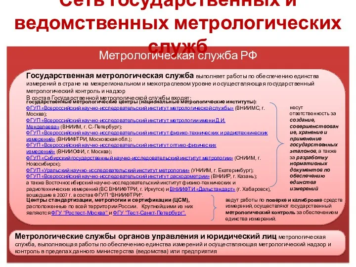 Сеть государственных и ведомственных метрологических служб
 Концепции управления персоналом
 Как правильно составить резюме
 Понятие и этапы планирования потребности в персонале
 Изменения порождают изменения
 Лекция 4. Раздел 2. Тема 2.1. Организация внешнего и внутреннего контроля
 Пути повышения производительности труда
 Основы деловой коммуникации. Как управлять деловым взаимодействием
 Взаимодействие организации с внешней средой
 Charting a company’s direction. Its vision, mission, objectives, and strategy. (Chapter 2)
 Власть и лидерство
 Стратегічне управління ресурсним потенціалом підприємства
 Роль логистики распределения в логистической системе
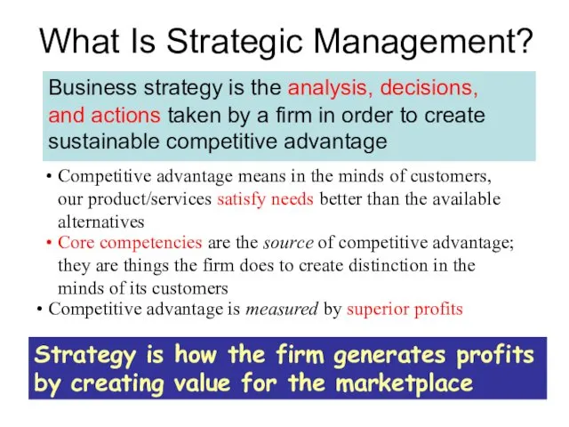 What Is Strategic Management?
 Способы предоставления продукции на контроль и методы сбора выборочной совокупности
 Диаграмма Исикавы. Рыбий скелет Исикавы
 Задачи управления запасами
 Типология управленческих решений и требования, предъявляемые к ним
 Личностные качества руководителя
 Отдельные улучшения, как важный элемент ТРМ
 Общество с ограниченной ответственностью МашИнКо
 Имидж и бренд СМИ. Связи с общественностью в редакционных структурах. (Тема 4)
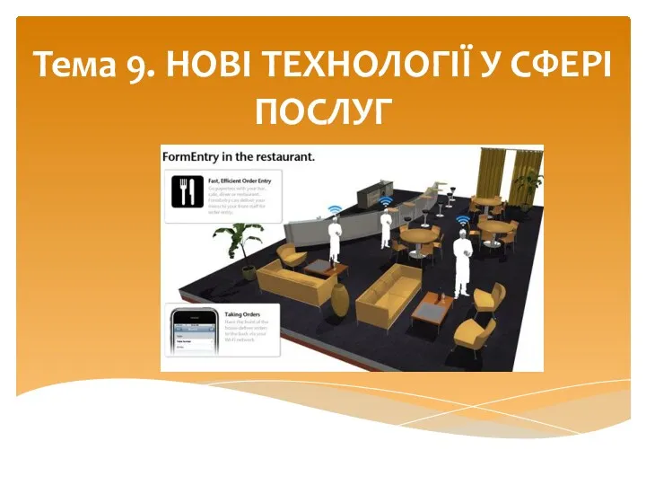 Нові технології у сфері послуг
 Классификация и характеристика моделей самооценки деятельности организации
 Оперативное хранение документов в текущей деятельности предприятия