- General terms of transmission lines performance and simulation

Содержание
- 2. Topics Power Systems Structure and Basic Elements AC Transmission Lines Modeling Classification Of Transmission Lines Typical
- 3. 1. Basic Circuit Elements
- 4. 1. Phasor Notation sinusoidally varying voltage is represented as an arrow of constant length, spinning around
- 5. 1. Power System Structure Main elements: 1. Generators; 2. Transformers; 3. Transmission lines.
- 6. 1. Control Structure Things we can control: Power flows; System frequency; Node voltages.
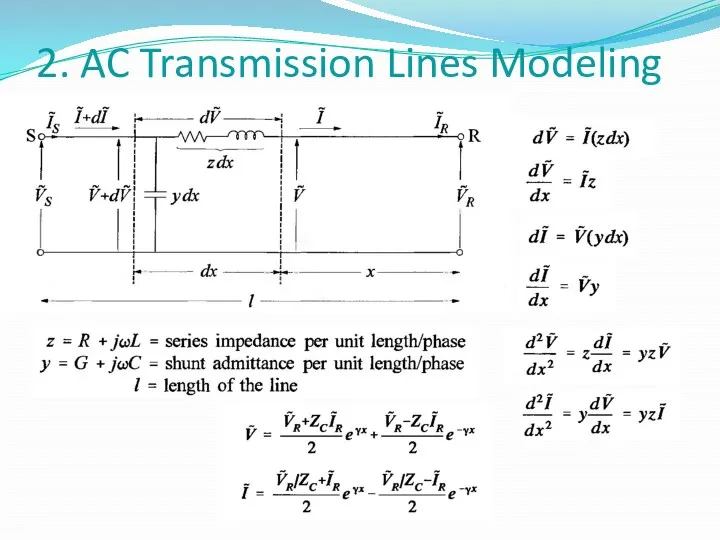
- 7. 2. AC Transmission Lines Modeling To develop performance equations and models for transmission lines; To examine
- 8. 2. AC Transmission Lines Modeling Series Resistance (R). The resistances of lines accounting for stranding and
- 9. 2. AC Transmission Lines Modeling AC transmission line tower construction defines its electric parameters. AC transmission
- 10. 2. AC Transmission Lines Modeling
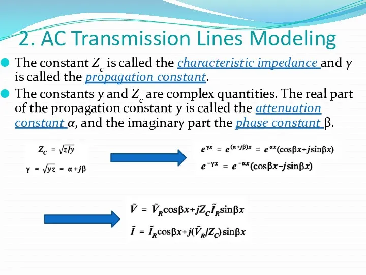
- 11. 2. AC Transmission Lines Modeling The constant Zc is called the characteristic impedance and γ is
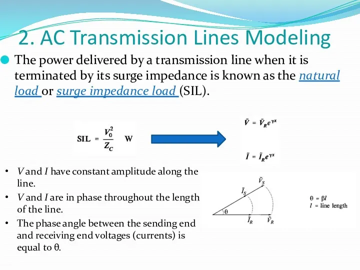
- 12. 2. AC Transmission Lines Modeling The power delivered by a transmission line when it is terminated
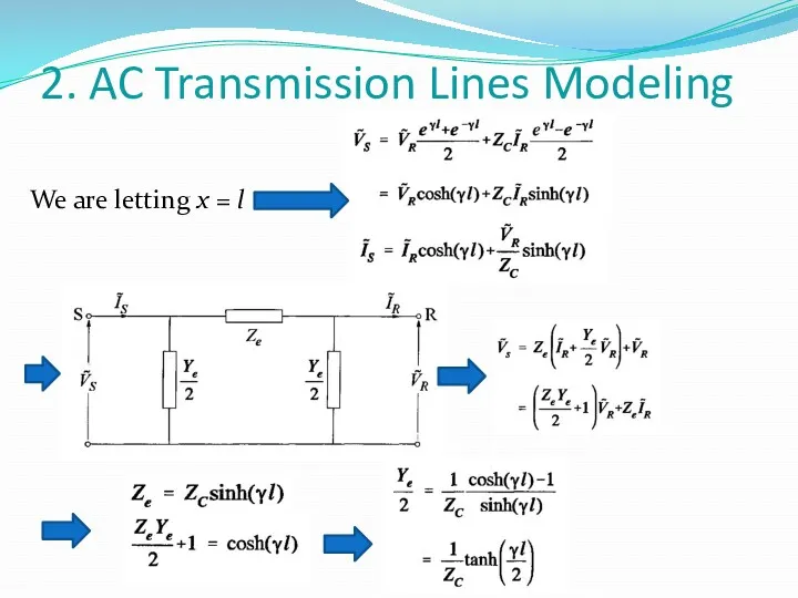
- 13. 2. AC Transmission Lines Modeling We are letting x = l
- 14. 3. Classification of TL by Length Short lines: lines shorter than about 100 km (60 mi).
- 15. 4. Typical Parameters
- 16. 5. Performance of a TL (no-load) (a) Receiving end is opened (IR=0) Neglecting losses Example: 300
- 17. 5. Performance of a TL (no-load) Voltage profile Current profile
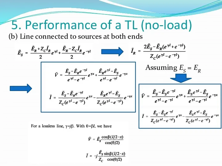
- 18. 5. Performance of a TL (no-load) (b) Line connected to sources at both ends Assuming ES
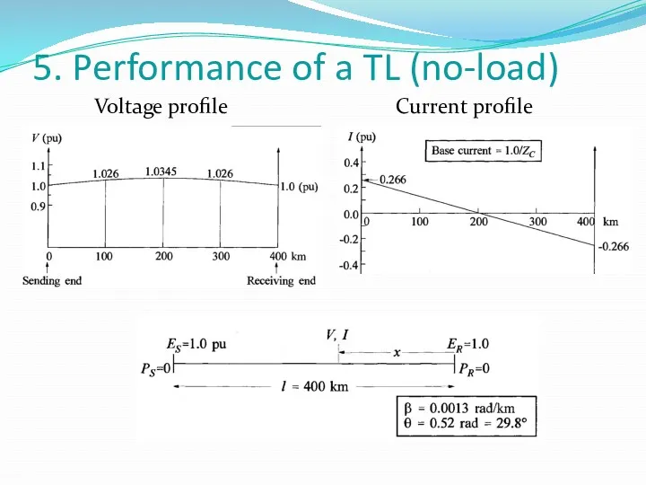
- 19. 5. Performance of a TL (no-load) Voltage profile Current profile
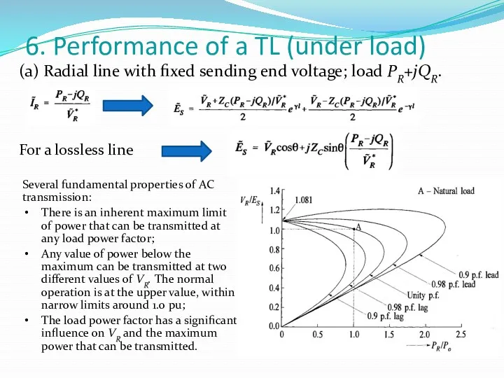
- 20. 6. Performance of a TL (under load) (a) Radial line with fixed sending end voltage; load
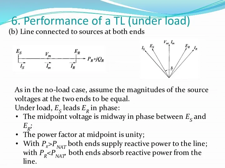
- 21. 6. Performance of a TL (under load) (b) Line connected to sources at both ends As
- 22. 7. Power Transfer and Stability Considerations Let δ be the angle by which ES leads ER
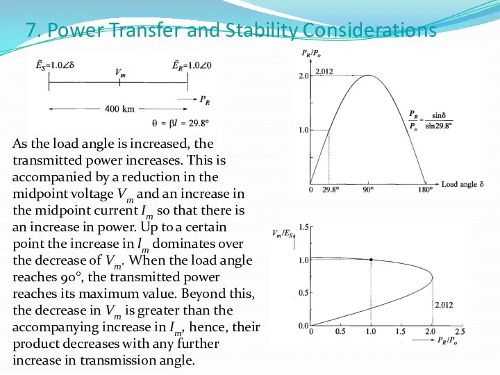
- 23. 7. Power Transfer and Stability Considerations As the load angle is increased, the transmitted power increases.
- 24. 8. Reactive Power Demand
- 25. 9. Tasks Using lossless line equations, solve the case for the line with fixed (known) sending
- 26. 10. Answers . . 1.4 pu. 0.31 pu, 600 Mvar Xmax = 214 km (from sending
- 28. Скачать презентацию
Topics
Power Systems Structure and Basic Elements
AC Transmission Lines Modeling
Classification Of Transmission
Topics
Power Systems Structure and Basic Elements
AC Transmission Lines Modeling
Classification Of Transmission
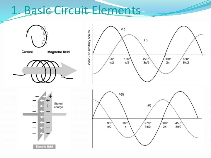
1. Basic Circuit Elements
1. Basic Circuit Elements
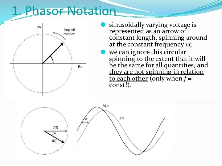
1. Phasor Notation
sinusoidally varying voltage is represented as an arrow of
1. Phasor Notation
sinusoidally varying voltage is represented as an arrow of
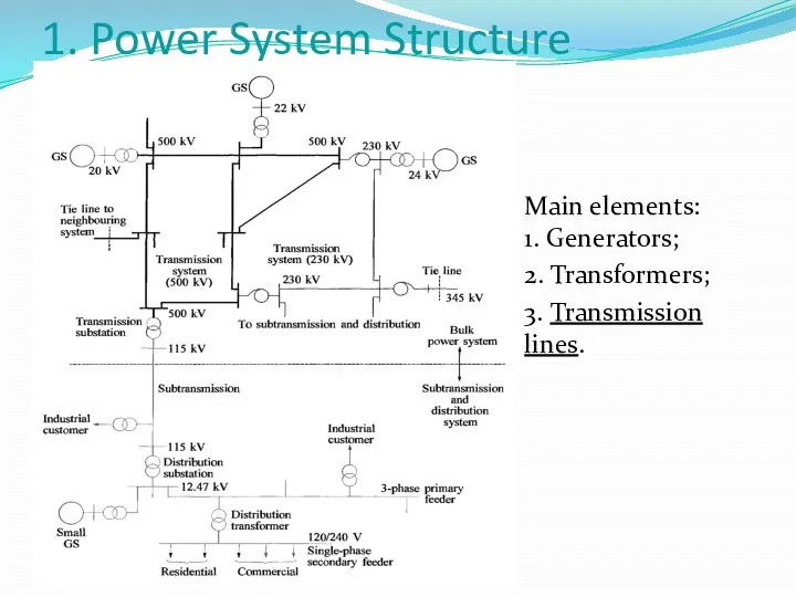
1. Power System Structure
Main elements:
1. Generators;
2. Transformers;
3. Transmission lines.
1. Power System Structure
Main elements:
1. Generators;
2. Transformers;
3. Transmission lines.
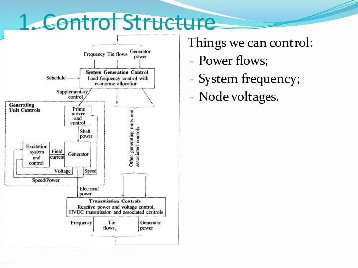
1. Control Structure
Things we can control:
Power flows;
System frequency;
Node voltages.
1. Control Structure
Things we can control:
Power flows;
System frequency;
Node voltages.
2. AC Transmission Lines Modeling
To develop performance equations and models for
2. AC Transmission Lines Modeling
To develop performance equations and models for
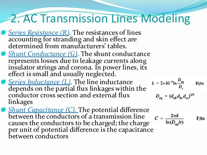
2. AC Transmission Lines Modeling
Series Resistance (R). The resistances of lines
2. AC Transmission Lines Modeling
Series Resistance (R). The resistances of lines
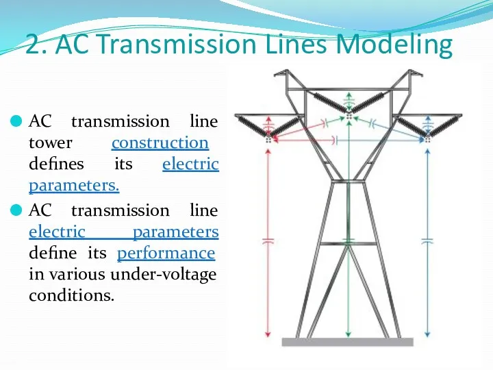
2. AC Transmission Lines Modeling
AC transmission line tower construction defines its
2. AC Transmission Lines Modeling
AC transmission line tower construction defines its
2. AC Transmission Lines Modeling
2. AC Transmission Lines Modeling
2. AC Transmission Lines Modeling
The constant Zc is called the characteristic
2. AC Transmission Lines Modeling
The constant Zc is called the characteristic
2. AC Transmission Lines Modeling
The power delivered by a transmission line
2. AC Transmission Lines Modeling
The power delivered by a transmission line
2. AC Transmission Lines Modeling
We are letting x = l
2. AC Transmission Lines Modeling
We are letting x = l
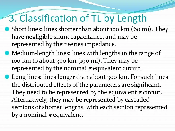
3. Classification of TL by Length
Short lines: lines shorter than about
3. Classification of TL by Length
Short lines: lines shorter than about
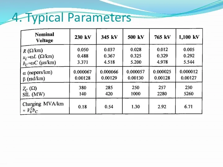
4. Typical Parameters
4. Typical Parameters
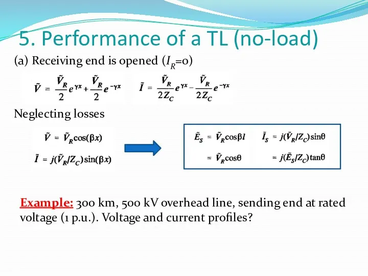
5. Performance of a TL (no-load)
(a) Receiving end is opened (IR=0)
Neglecting
5. Performance of a TL (no-load)
(a) Receiving end is opened (IR=0)
Neglecting
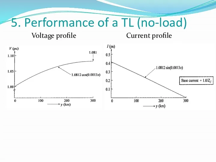
5. Performance of a TL (no-load)
Voltage profile
Current profile
5. Performance of a TL (no-load)
Voltage profile
Current profile
5. Performance of a TL (no-load)
(b) Line connected to sources at
5. Performance of a TL (no-load)
(b) Line connected to sources at
5. Performance of a TL (no-load)
Voltage profile
Current profile
5. Performance of a TL (no-load)
Voltage profile
Current profile
6. Performance of a TL (under load)
(a) Radial line with fixed
6. Performance of a TL (under load)
(a) Radial line with fixed
6. Performance of a TL (under load)
(b) Line connected to sources
6. Performance of a TL (under load)
(b) Line connected to sources
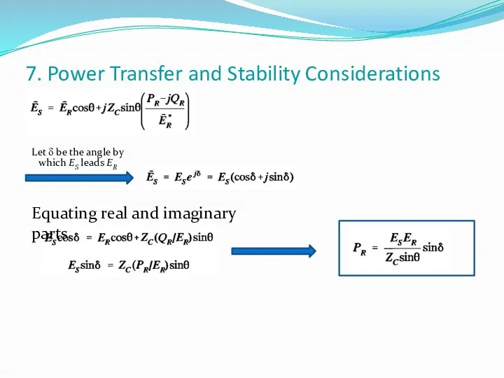
7. Power Transfer and Stability Considerations
Let δ be the angle by
7. Power Transfer and Stability Considerations
Let δ be the angle by
7. Power Transfer and Stability Considerations
As the load angle is increased,
7. Power Transfer and Stability Considerations
As the load angle is increased,
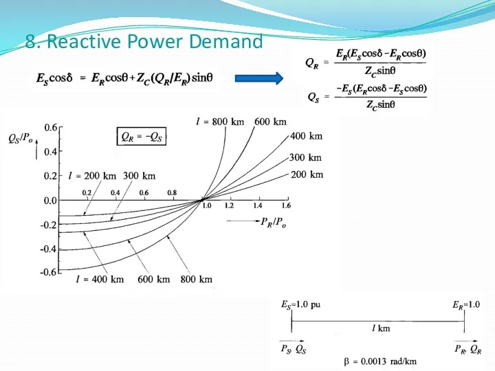
8. Reactive Power Demand
8. Reactive Power Demand
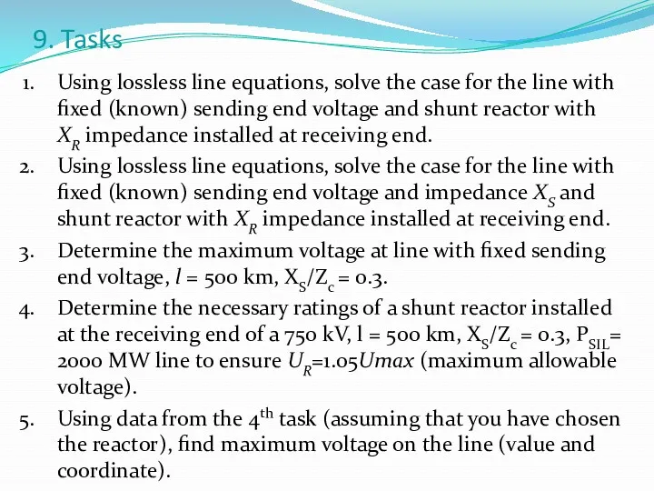
9. Tasks
Using lossless line equations, solve the case for the line
9. Tasks
Using lossless line equations, solve the case for the line
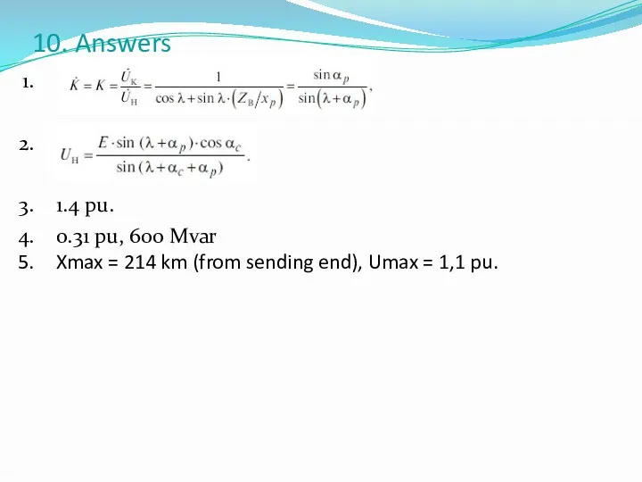
10. Answers
.
.
1.4 pu.
0.31 pu, 600 Mvar
Xmax = 214 km (from sending
10. Answers
.
.
1.4 pu.
0.31 pu, 600 Mvar
Xmax = 214 km (from sending
Похожие презентации
 Интеллектуальный марафон - 13 (2 класс)
 Текст и предложение
 Лазерные технологии в амбулаторной оториноларингологии
 Религия иудаизм
 Пулковский рубеж
 5 класс 5.02
 Образовательные программы учащихся с ОВЗ и инвалидностью – требования, структура, условия реализации в разных формах
 Отчет по производственной практике Информационные системы
 Конспект интегрированного логопедического занятия Времена года, круговорот воды в природе и безударные гласные
 Центробежный насос
 Ведение мяча и броски
 Белый цвет. Снеговик
 Презентация Технологии деятельностного типа применяемые при изучении химии.
 Урок Простые вещества
 Проектирование индивидуального образовательного маршрута сопровождения детей в рамках ПМПк
 Презентация Трудности адаптации ребенка в 5 классе
 Плазменная обработка. Технологии в современном мире
 Общие сведения о пунктах управления подразделениями ПВО мсп (тп) и омсбр (отбр). Занятие №1
 Легендарная Пирятинская
 Электрооборудование карьерных подстанций
 Котельные установки и парогенераторы. Часть 2. Лекции 7 - 8
 Метод наглядного моделирования как средство развития связной речи у детей дошкольного возраста
 Лесные культуры
 Примерная структура планирования воспитательно-образовательной работы на 1 день
 Основные дефекты строительных конструкций
 Сравнительно-сопоставительный анализ якутского и алтайского шаманизма
 Принципы проведения референдума. Вопросы референдума и порядок их вынесения