- Long-Range Order and Superconductivity

Содержание
- 2. Density matrix in quantum mechanics If one has a large closed quantum-mechanical system with co-ordinates q
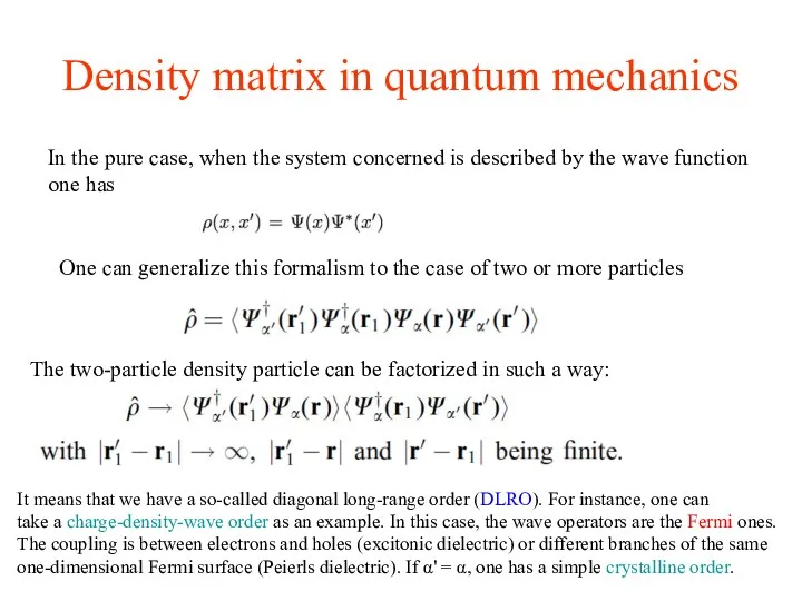
- 3. Density matrix in quantum mechanics In the pure case, when the system concerned is described by
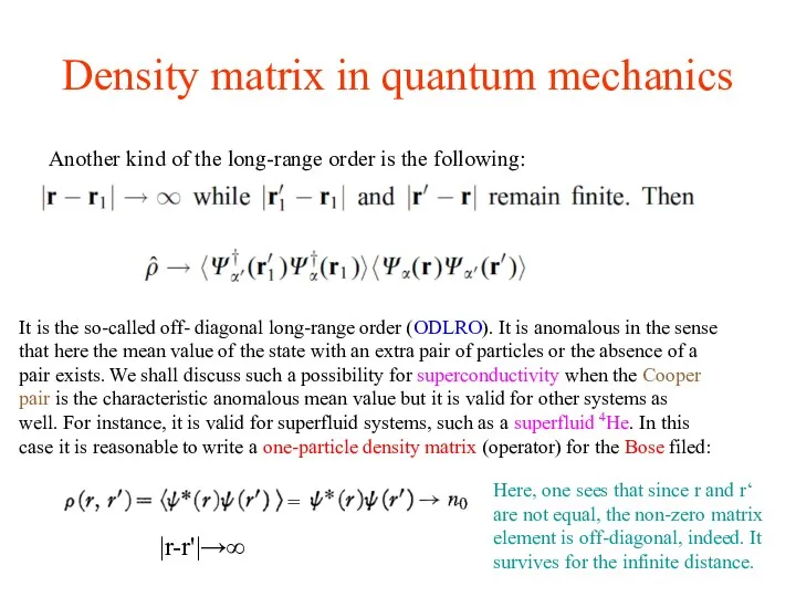
- 4. Density matrix in quantum mechanics Another kind of the long-range order is the following: It is
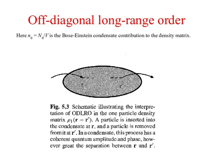
- 5. Off-diagonal long-range order Here n0 = N0/V is the Bose-Einstein condensate contribution to the density matrix.
- 6. Long-range orders below critical lines of phase transitions (4He)
- 7. Phase transitions This is the phenomenological way to describe all kinds of phase transitions. It was
- 8. MICHAEL FARADAY, THE PRECURSOR OF LIQUEFACTION Michael Faraday, 1791-1867 He liquefied all gases known to him
- 9. JAMES DEWAR, THE COMPETITOR – A MAN, WHO LIQUEFIED HYDROGEN IN 1898 A Dewar flask in
- 10. KAMERLINGH-ONNES, THE WINNER – PHYSICIST AND ENGINEER (Nobel Prize in Physics, 1913) Heike Kamerlingh Onnes (right)
- 11. LOW TEMPERATURE STUDIES USING LIQUID HELIUM LED TO NEW DISCOVERIES: NOT ONLY SUPERCONDUCTIVITY! Phase transition in
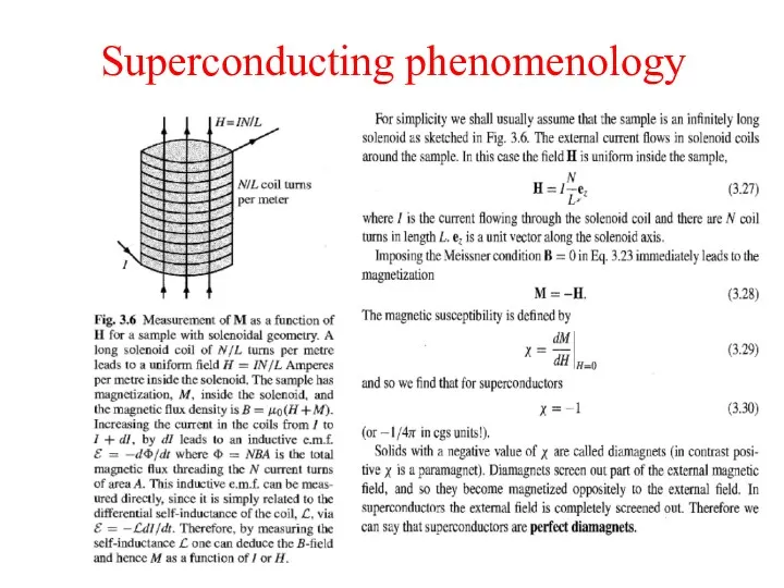
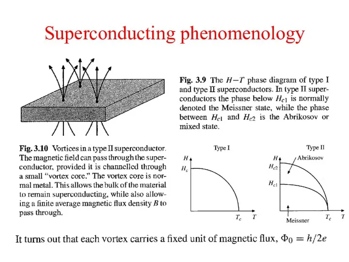
- 12. Superconducting phenomenology
- 13. SUPERCONDUCTIVITY AMONG ELEMENTS
- 14. SUPERCONDUCTIVITY, A MIRACLE FOUND BY KAMERLINGH-ONNES Superconducting levitation based on Meissner effect
- 15. ANNIVERSARIES OF key discoveries 1908-2008 (100) Helium liquefying 1911-2011 (100) Superconductivity 1933-2013 (70) Meissner-Ochsenfeld effect 1956-2011
- 16. PHENOMENOLOGY. NORMAL METALS
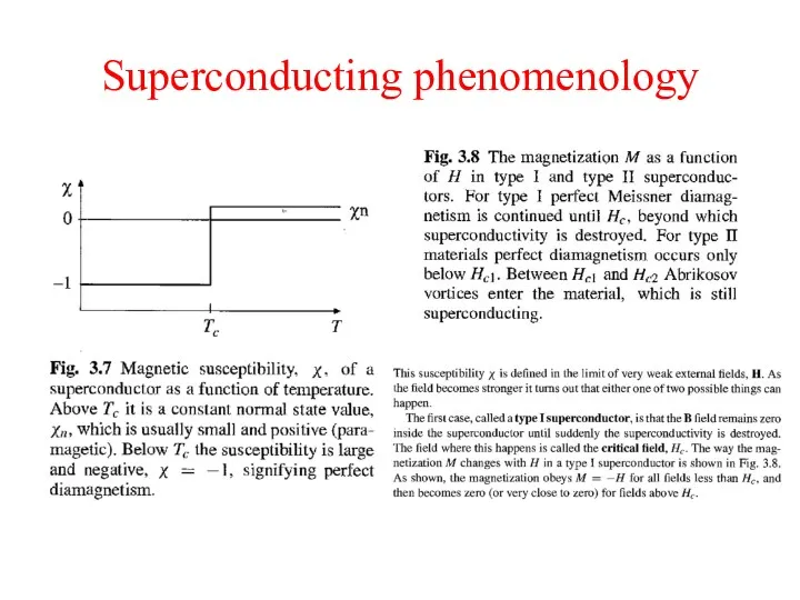
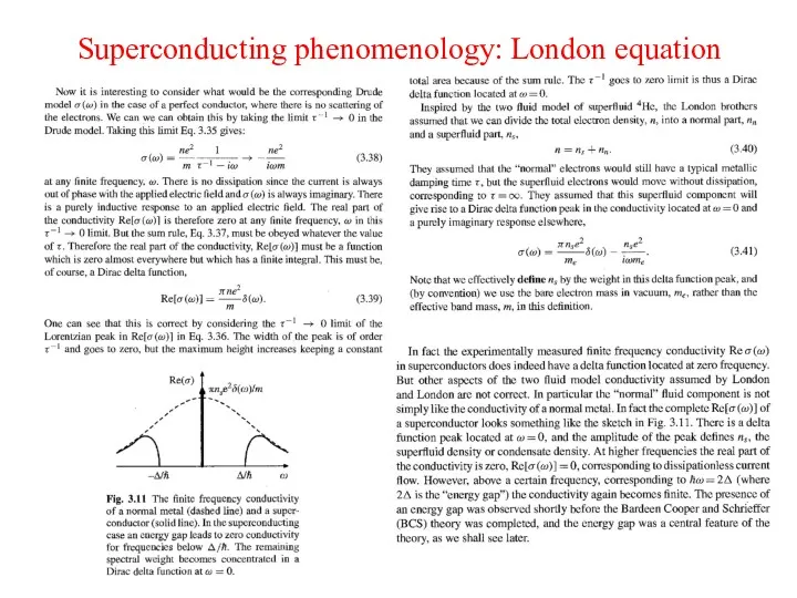
- 17. Superconducting phenomenology
- 18. Magnetic field, magnetic induction, and magnetization
- 19. Superconducting phenomenology
- 20. Superconducting phenomenology
- 21. Superconducting phenomenology We define the magnetic field H in terms of the external currents only
- 22. Superconducting phenomenology
- 23. Superconducting phenomenology
- 24. Creators of the type II superconductors A. A. Abrikosov
- 25. Superconducting phenomenology
- 26. Superconducting phenomenology
- 27. Superconducting phenomenology: London equation We This model leads to the famous London equation Here, j is
- 28. Superconducting phenomenology: London equation
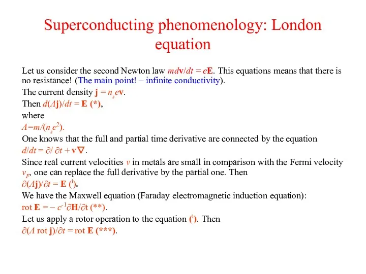
- 29. Superconducting phenomenology: London equation Let us consider the second Newton law mdv/dt = eE. This equations
- 30. Superconducting phenomenology: London equation From (**) and (***) one obtains ∂(Λ rot j)/∂t = − c-1∂H/∂t
- 31. Superconducting phenomenology: London equation Equation (*****) and the Maxwell equation rot H = 4πj/c leads to
- 32. Superconducting phenomenology: London equation From (3.48) and Eq. (*****) one obtains
- 33. Superconducting phenomenology: London equation We saw that the suggestions j = 0 and H = 0
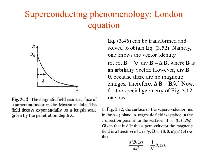
- 34. Superconducting phenomenology: London equation Eq. (3.46) can be transformed and solved to obtain Eq. (3.52). Namely,
- 35. Superconducting phenomenology: London equation
- 36. Superconducting phenomenology: London-Pippard equation
- 37. Brian Pippard (1920-2008)
- 38. Superconducting phenomenology: London-Pippard equation
- 39. Superconductors of the first and second kind
- 40. Superconductors of the first and second kind
- 42. Скачать презентацию
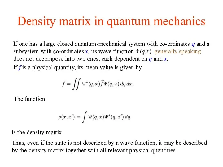
Density matrix in quantum mechanics
If one has a large closed quantum-mechanical
Density matrix in quantum mechanics
If one has a large closed quantum-mechanical
Density matrix in quantum mechanics
In the pure case, when the system
Density matrix in quantum mechanics
In the pure case, when the system
Density matrix in quantum mechanics
Another kind of the long-range order is
Density matrix in quantum mechanics
Another kind of the long-range order is
Off-diagonal long-range order
Here n0 = N0/V is the Bose-Einstein condensate contribution
Off-diagonal long-range order
Here n0 = N0/V is the Bose-Einstein condensate contribution
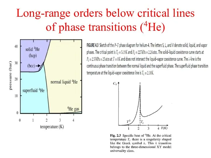
Long-range orders below critical lines of phase transitions (4He)
Long-range orders below critical lines of phase transitions (4He)
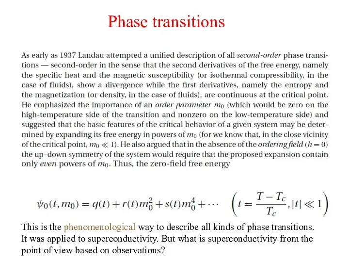
Phase transitions
This is the phenomenological way to describe all kinds of
Phase transitions
This is the phenomenological way to describe all kinds of
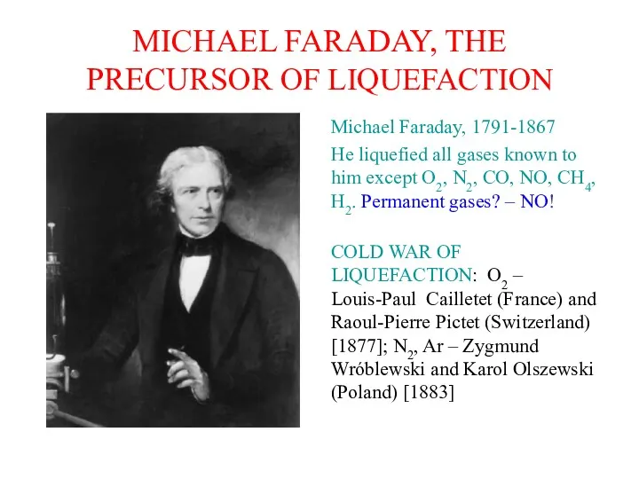
MICHAEL FARADAY, THE PRECURSOR OF LIQUEFACTION
Michael Faraday, 1791-1867
He liquefied all gases
MICHAEL FARADAY, THE PRECURSOR OF LIQUEFACTION
Michael Faraday, 1791-1867
He liquefied all gases
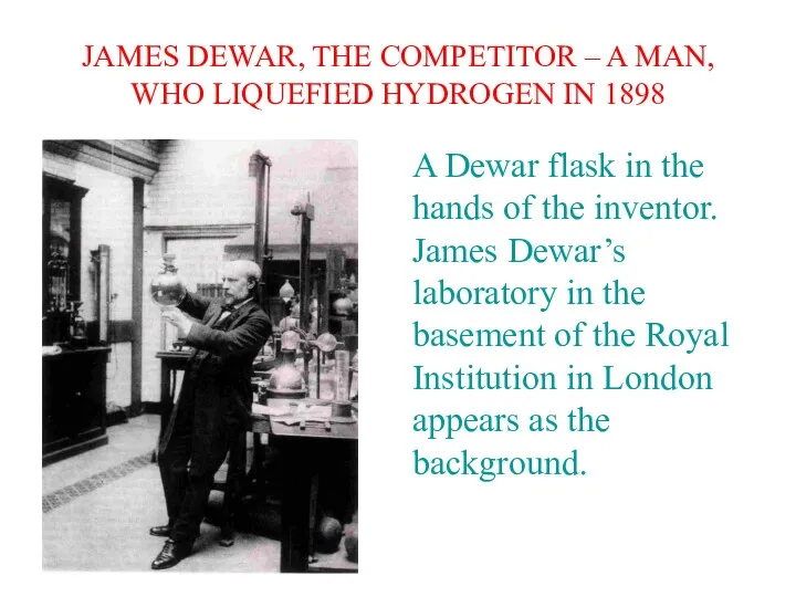
JAMES DEWAR, THE COMPETITOR – A MAN, WHO LIQUEFIED HYDROGEN IN
JAMES DEWAR, THE COMPETITOR – A MAN, WHO LIQUEFIED HYDROGEN IN
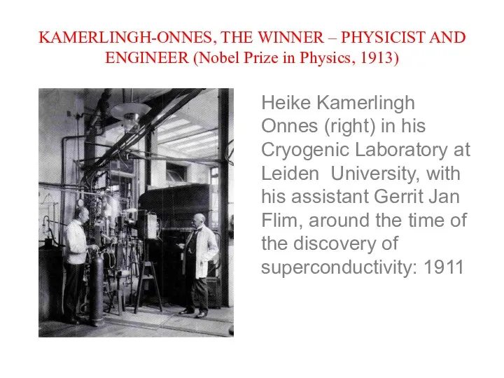
KAMERLINGH-ONNES, THE WINNER – PHYSICIST AND ENGINEER (Nobel Prize in Physics,
KAMERLINGH-ONNES, THE WINNER – PHYSICIST AND ENGINEER (Nobel Prize in Physics,
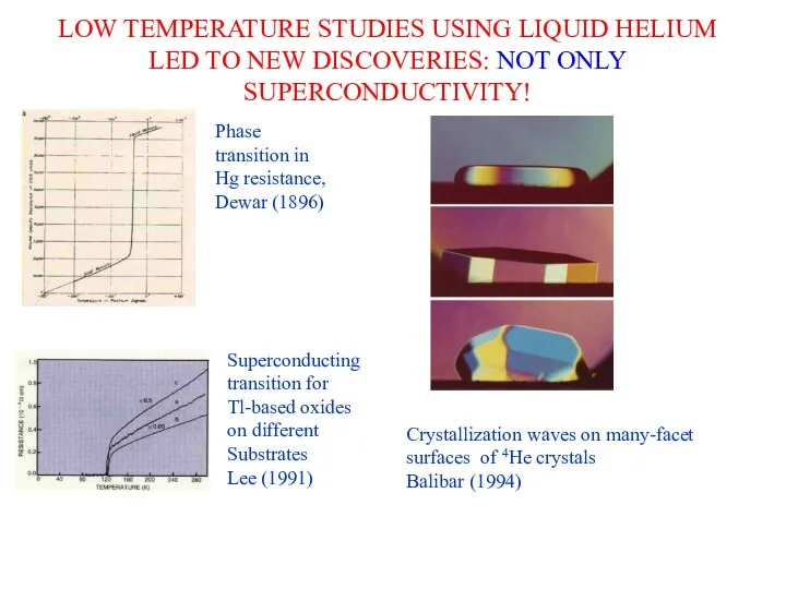
LOW TEMPERATURE STUDIES USING LIQUID HELIUM LED TO NEW DISCOVERIES: NOT
LOW TEMPERATURE STUDIES USING LIQUID HELIUM LED TO NEW DISCOVERIES: NOT
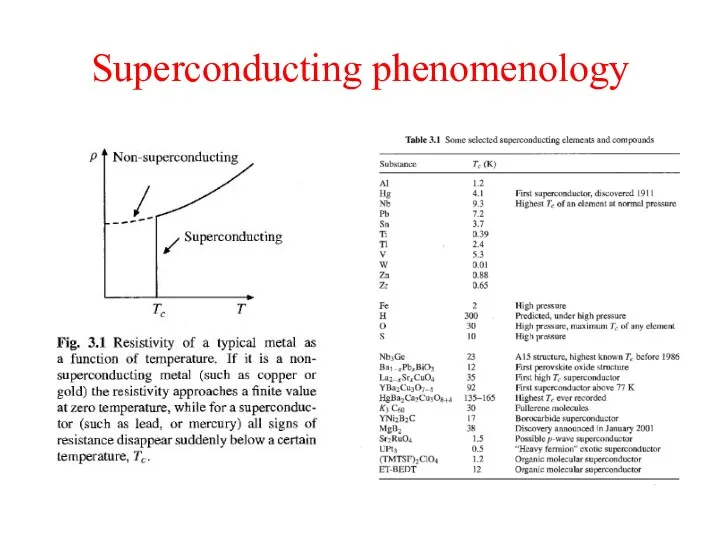
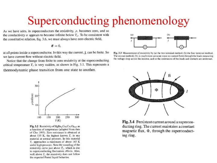
Superconducting phenomenology
Superconducting phenomenology
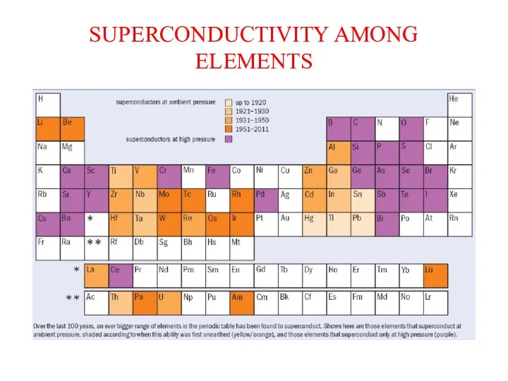
SUPERCONDUCTIVITY AMONG ELEMENTS
SUPERCONDUCTIVITY AMONG ELEMENTS
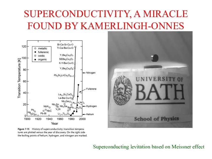
SUPERCONDUCTIVITY, A MIRACLE FOUND BY KAMERLINGH-ONNES
Superconducting levitation based on Meissner effect
SUPERCONDUCTIVITY, A MIRACLE FOUND BY KAMERLINGH-ONNES
Superconducting levitation based on Meissner effect
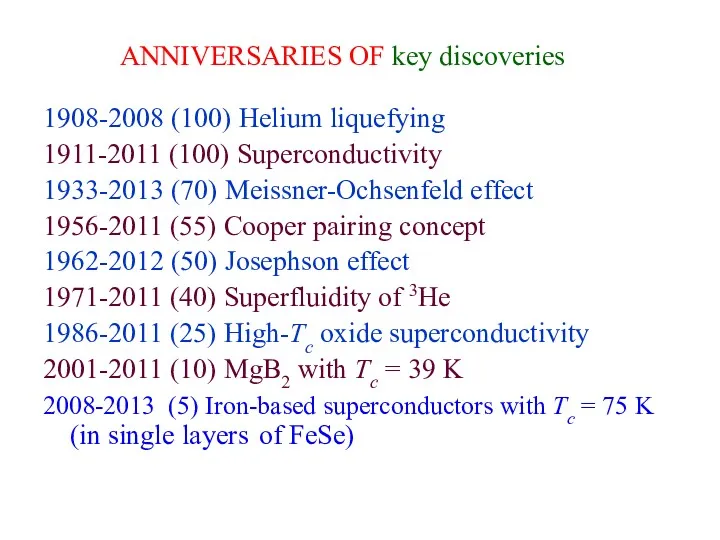
ANNIVERSARIES OF key discoveries
1908-2008 (100) Helium liquefying
1911-2011 (100) Superconductivity
1933-2013 (70) Meissner-Ochsenfeld
ANNIVERSARIES OF key discoveries
1908-2008 (100) Helium liquefying
1911-2011 (100) Superconductivity
1933-2013 (70) Meissner-Ochsenfeld
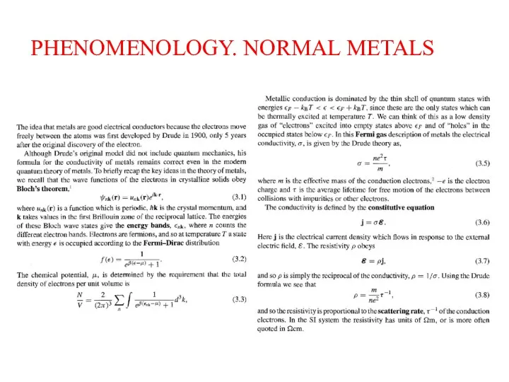
PHENOMENOLOGY. NORMAL METALS
PHENOMENOLOGY. NORMAL METALS
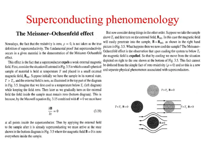
Superconducting phenomenology
Superconducting phenomenology
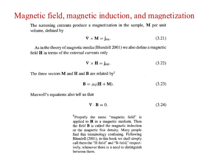
Magnetic field, magnetic induction, and magnetization
Magnetic field, magnetic induction, and magnetization
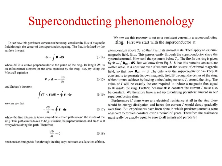
Superconducting phenomenology
Superconducting phenomenology
Superconducting phenomenology
Superconducting phenomenology
Superconducting phenomenology
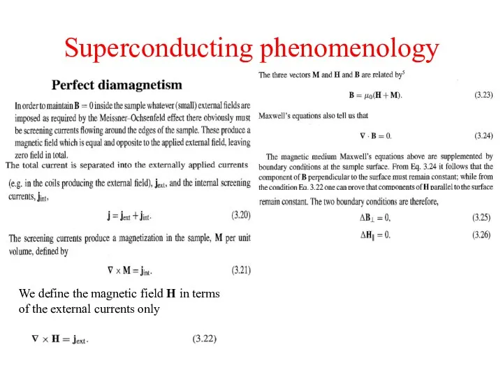
We define the magnetic field H in terms
of the
Superconducting phenomenology
We define the magnetic field H in terms
of the
Superconducting phenomenology
Superconducting phenomenology
Superconducting phenomenology
Superconducting phenomenology
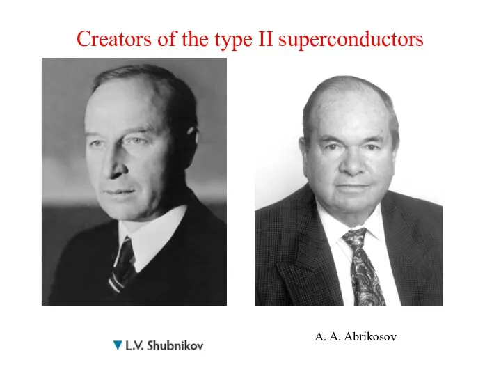
Creators of the type II superconductors
A. A. Abrikosov
Creators of the type II superconductors
A. A. Abrikosov
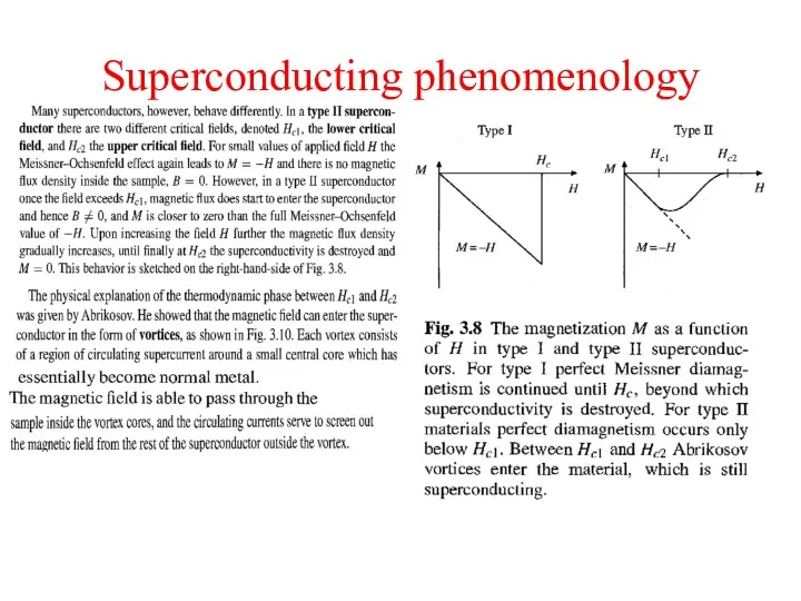
Superconducting phenomenology
Superconducting phenomenology
Superconducting phenomenology
Superconducting phenomenology
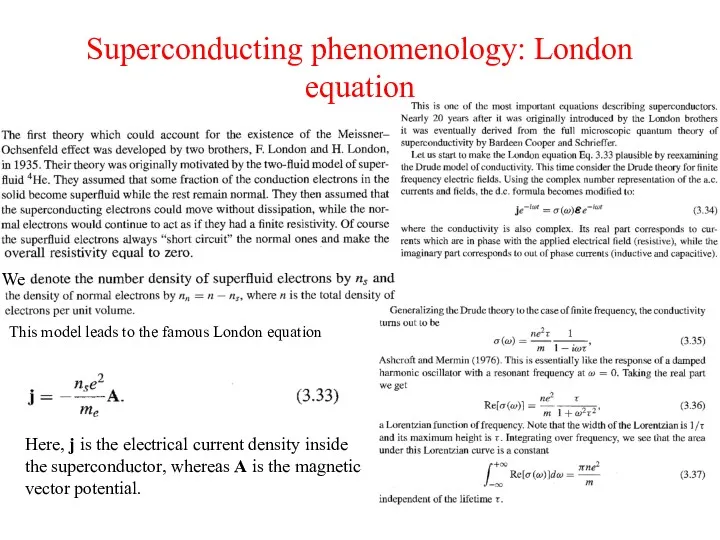
Superconducting phenomenology: London equation
We
This model leads to the famous London equation
Here,
Superconducting phenomenology: London equation
We
This model leads to the famous London equation
Here,
Superconducting phenomenology: London equation
Superconducting phenomenology: London equation
Superconducting phenomenology: London equation
Let us consider the second Newton law mdv/dt
Superconducting phenomenology: London equation
Let us consider the second Newton law mdv/dt
Superconducting phenomenology: London equation
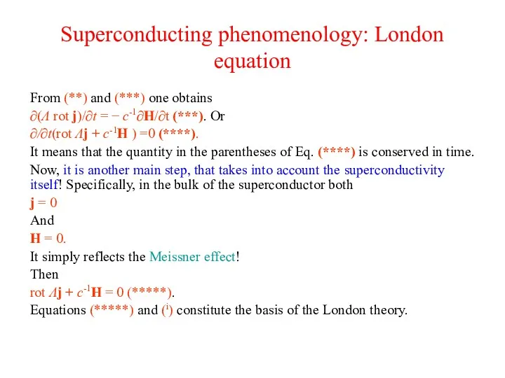
From (**) and (***) one obtains
∂(Λ rot j)/∂t
Superconducting phenomenology: London equation
From (**) and (***) one obtains
∂(Λ rot j)/∂t
Superconducting phenomenology: London equation
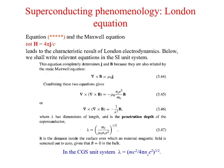
Equation (*****) and the Maxwell equation
rot H =
Superconducting phenomenology: London equation
Equation (*****) and the Maxwell equation
rot H =
Superconducting phenomenology: London equation
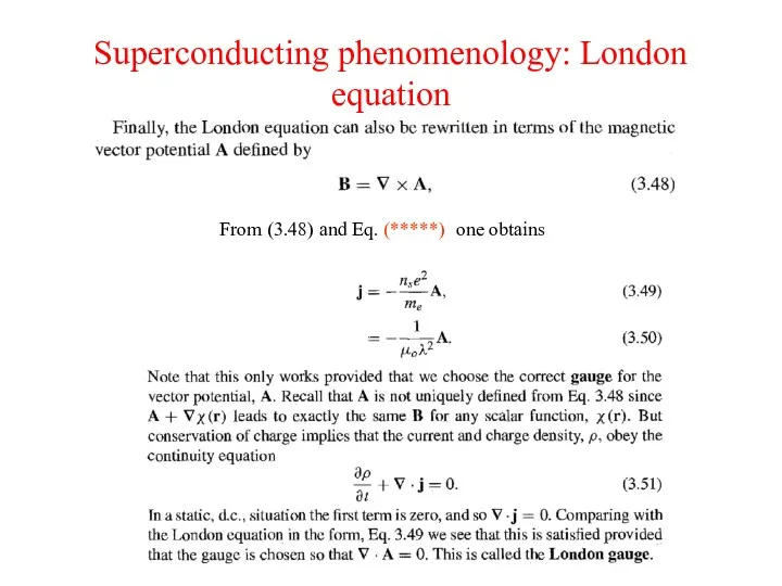
From (3.48) and Eq. (*****) one obtains
Superconducting phenomenology: London equation
From (3.48) and Eq. (*****) one obtains
Superconducting phenomenology: London equation
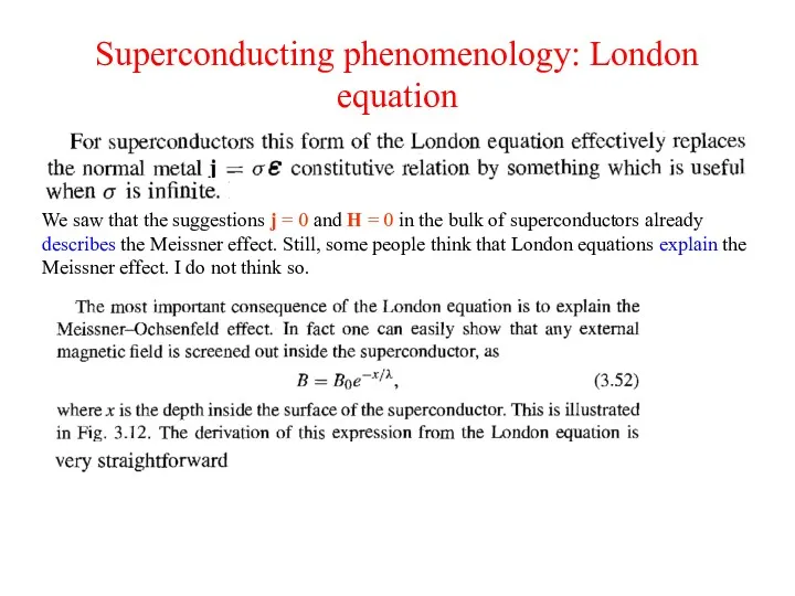
We saw that the suggestions j = 0
Superconducting phenomenology: London equation
We saw that the suggestions j = 0
Superconducting phenomenology: London equation
Eq. (3.46) can be transformed and solved to
Superconducting phenomenology: London equation
Eq. (3.46) can be transformed and solved to
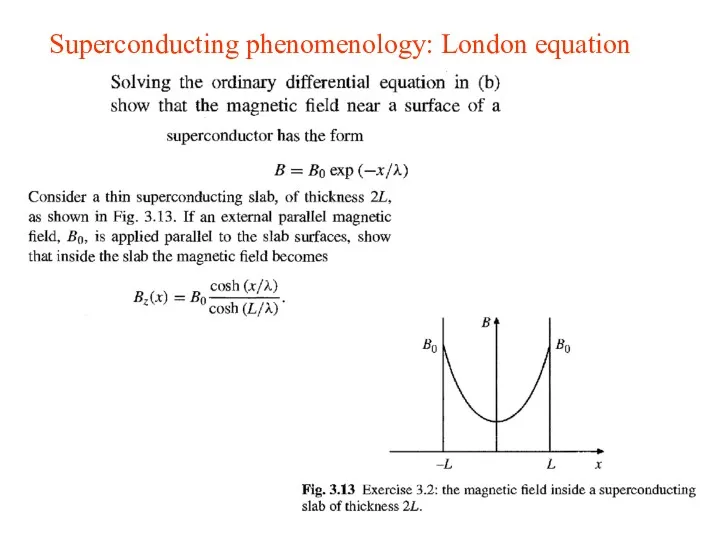
Superconducting phenomenology: London equation
Superconducting phenomenology: London equation
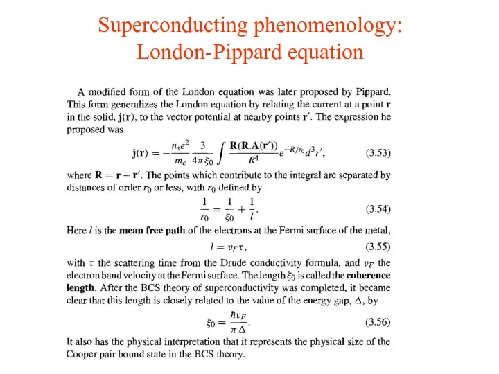
Superconducting phenomenology: London-Pippard equation
Superconducting phenomenology: London-Pippard equation
Brian Pippard (1920-2008)
Brian Pippard (1920-2008)
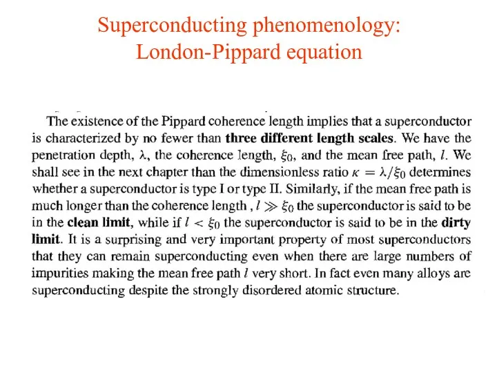
Superconducting phenomenology: London-Pippard equation
Superconducting phenomenology: London-Pippard equation

Superconductors of the first and second kind
Superconductors of the first and second kind
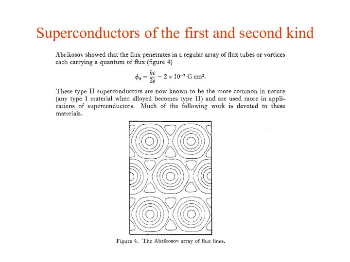
Superconductors of the first and second kind
Superconductors of the first and second kind
 Семинар для воспитателей Интонационная сторона речи дошкольников
 Интеллектуальная игра Брей-ринг
 Компьютерно -игровая зависимость и её профилактика.
 Игра-викторина. Вопросики
 Теплоэнергетика технологии обжига известняка во вращающихся печах
 Direkt Subjekt + Prädikat + Nebenglieder Ich lerne Deutsch nicht lange
 Человек и домашние животные
 Электрооборудование общепромышленных установок
 Родительское собрание №1. 2 класс
 Разработка и исследование регулируемого электропривода механизма подъема лебедки мостового крана грузоподъемностью 50 т
 Система сбалансированных показателей. Показатели стратегических финансовых направлений
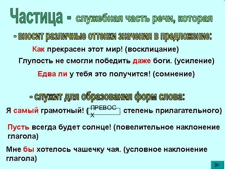 Формообразующие частицы
 Эдуард Анатольевич Стрельцов,
 Острый и хронический синусит
 Буквы Е, Ё, Ю, Я и их функции в словах
 Поверхностное упрочнение стальных деталей
 Гликоген. Структура. Физические и химические свойства
 Презентація
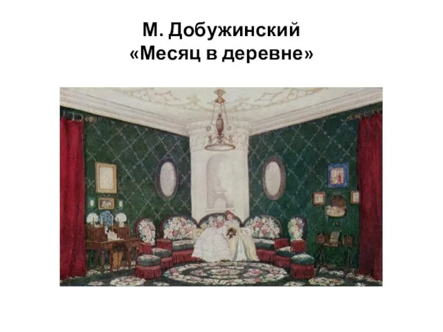 Художник и театр
 Ванты. вантовые конструкции
 Снятие мерок с фигуры человека
 История обыкновенных дробей
 Забытая война, посвященный 100-летию начала Первой мировой войны
 Особенности ВНД человека. Познавательные процессы
 Фосфор
 Совет Лицеистов
 Работы учащихся 9 классов ГБОУ СОШ 599 (презентации к уроку)
 Защита у организмов