- Particle Size Analysis

Содержание
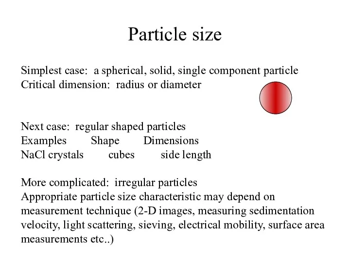
- 2. Particle size Simplest case: a spherical, solid, single component particle Critical dimension: radius or diameter Next
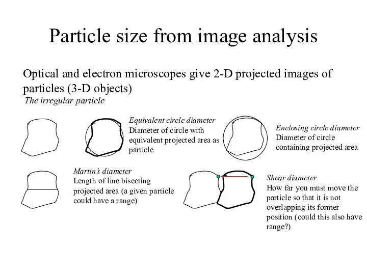
- 3. Particle size from image analysis Optical and electron microscopes give 2-D projected images of particles (3-D
- 4. “The Radius of Gyration of an Area about a given axis is a distance k from
- 5. Diameters can vary, exercise
- 6. Particle size- equivalent diameters Other equivalent diameters can be defined: Sieve equivalent diameter – diameter equal
- 7. More diameters Volume diameter – diameter of sphere having same volume Obtained from Coulter counter techniques
- 9. Concept of fractal dimension Aerosol particles which consist of agglomerates of ‘primary particles’, (often, combustion generated)
- 10. Fractal dimension Fractals - Df = 2 = uniform density in a plane, Df of 3
- 11. Particle Size Con’t Particle concentration – suspensions in air Particle density – powders What if particles
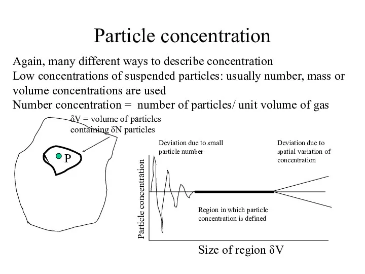
- 12. Particle concentration Again, many different ways to describe concentration Low concentrations of suspended particles: usually number,
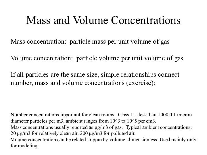
- 13. Mass and Volume Concentrations Mass concentration: particle mass per unit volume of gas Volume concentration: particle
- 14. Particle concentrations - powders Additional definitions necessary: Bed or bulk density = mass of particles in
- 15. What if we have a mixture of particles of different sizes? In the real world, this
- 16. Example histogram: Can also create histogram from raw particle size data using Analysis tool pack add-in,
- 17. Continuous particle size distributions More useful: continuous distributions, where some function, nd, describes the number of
- 18. More continuous size distributions M is total mass of particles per unit volume at a given
- 19. What do they look like?
- 20. Frequency distributions Cumulative frequency distribution: FN = fraction of number of particles with diameter (Fv for
- 21. Example of cumulative frequency distribution from discrete data Example of differential frequency distribution in Fig. 3.3
- 22. More on size distributions In measuring size distributions, instruments such as impactors give mass of particles
- 23. Spreadsheet tricks
- 24. Number, mass, surface area distributions not the same! Mass distribution from before Using arithmetic average of
- 25. Describing distributions using a single number, a.k.a. what is average? General formula for the mean, x,
- 26. Standard shapes of distributions Normal Log normal Bimodal
- 27. Similarity transformation The similarity transformation for the particle size distribution is based on the assumption that
- 28. Self-preserving size distribution For simplest case: no material added or lost from the system, V is
- 30. Скачать презентацию
Particle size
Simplest case: a spherical, solid, single component particle
Critical dimension:
Particle size
Simplest case: a spherical, solid, single component particle
Critical dimension:
Particle size from image analysis
Optical and electron microscopes give 2-D projected
Particle size from image analysis
Optical and electron microscopes give 2-D projected
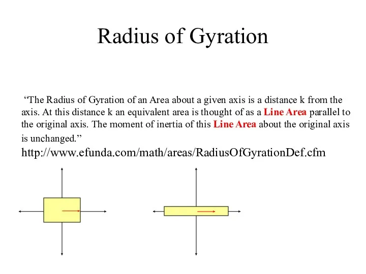
“The Radius of Gyration of an Area about a given
“The Radius of Gyration of an Area about a given
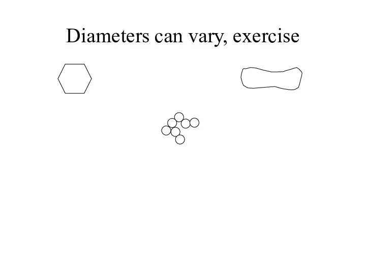
Diameters can vary, exercise
Diameters can vary, exercise
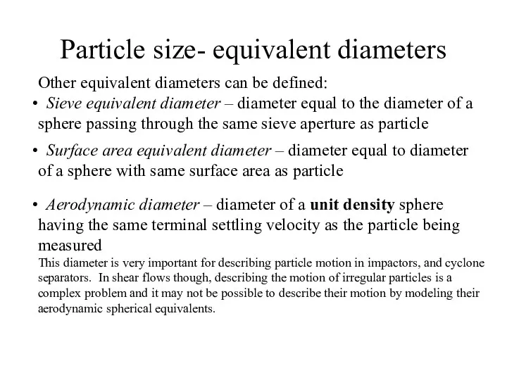
Particle size- equivalent diameters
Other equivalent diameters can be defined:
Sieve
Particle size- equivalent diameters
Other equivalent diameters can be defined:
Sieve
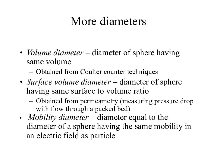
More diameters
Volume diameter – diameter of sphere having same volume
Obtained from
More diameters
Volume diameter – diameter of sphere having same volume
Obtained from
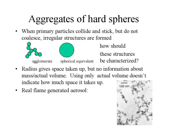
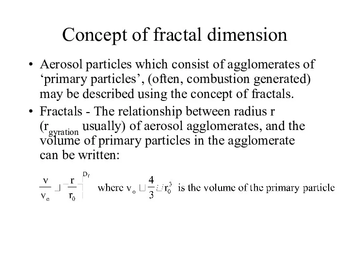
Concept of fractal dimension
Aerosol particles which consist of agglomerates of ‘primary
Concept of fractal dimension
Aerosol particles which consist of agglomerates of ‘primary
Fractal dimension
Fractals - Df = 2 = uniform density in a
Fractal dimension
Fractals - Df = 2 = uniform density in a
Particle Size Con’t
Particle concentration – suspensions in air
Particle density – powders
What
Particle Size Con’t
Particle concentration – suspensions in air
Particle density – powders
What
Particle concentration
Again, many different ways to describe concentration
Low concentrations of suspended
Particle concentration
Again, many different ways to describe concentration
Low concentrations of suspended
Mass and Volume Concentrations
Mass concentration: particle mass per unit volume of
Mass and Volume Concentrations
Mass concentration: particle mass per unit volume of
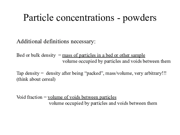
Particle concentrations - powders
Additional definitions necessary:
Bed or bulk density =
Particle concentrations - powders
Additional definitions necessary:
Bed or bulk density =
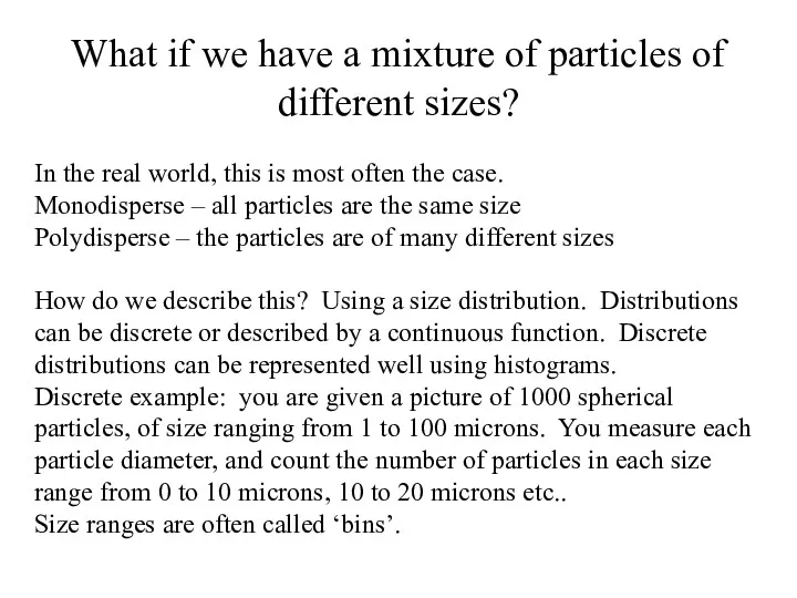
What if we have a mixture of particles of different sizes?
What if we have a mixture of particles of different sizes?
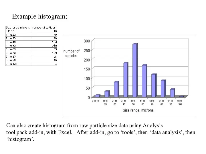
Example histogram:
Can also create histogram from raw particle size data
Example histogram:
Can also create histogram from raw particle size data
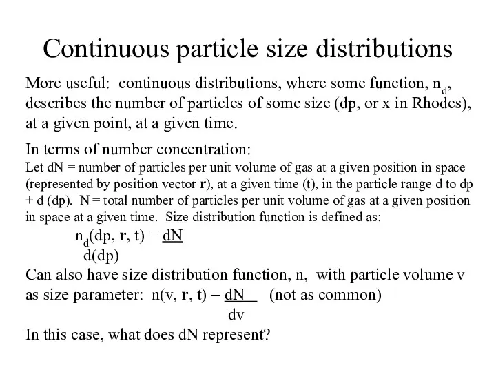
Continuous particle size distributions
More useful: continuous distributions, where some function, nd,
Continuous particle size distributions
More useful: continuous distributions, where some function, nd,
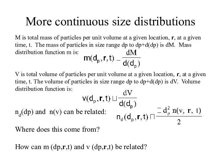
More continuous size distributions
M is total mass of particles per
More continuous size distributions
M is total mass of particles per
What do they look like?
What do they look like?
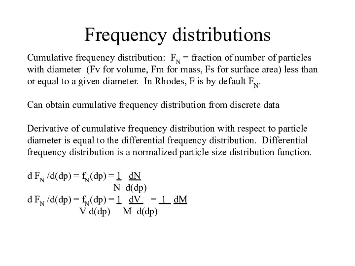
Frequency distributions
Cumulative frequency distribution: FN = fraction of number of particles
Frequency distributions
Cumulative frequency distribution: FN = fraction of number of particles
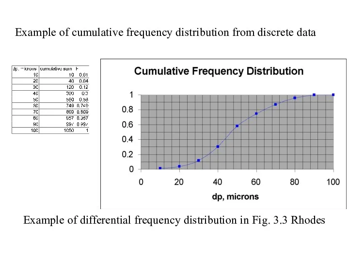
Example of cumulative frequency distribution from discrete data
Example of differential frequency
Example of cumulative frequency distribution from discrete data
Example of differential frequency
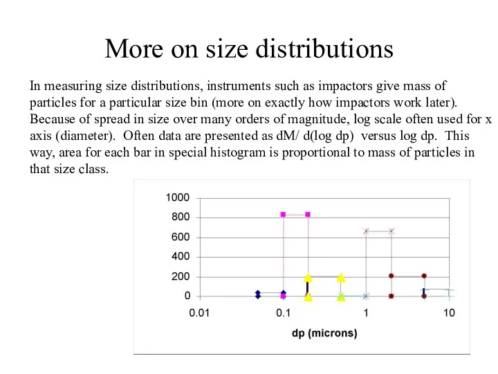
More on size distributions
In measuring size distributions, instruments such as impactors
More on size distributions
In measuring size distributions, instruments such as impactors
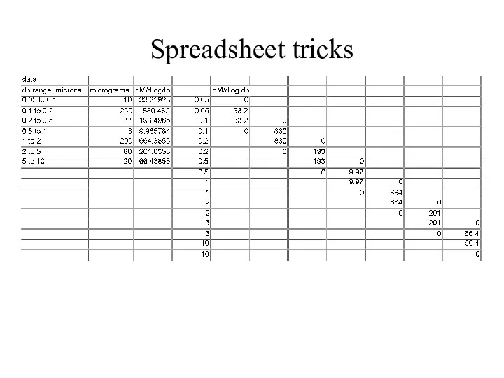
Spreadsheet tricks
Spreadsheet tricks
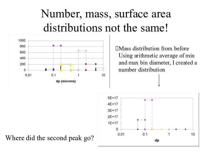
Number, mass, surface area distributions not the same!
Mass distribution from before
Using
Number, mass, surface area distributions not the same!
Mass distribution from before
Using
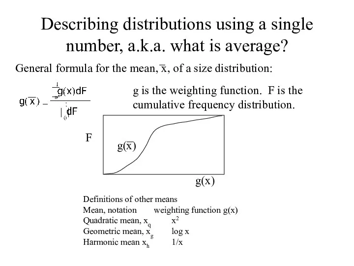
Describing distributions using a single number, a.k.a. what is average?
General
Describing distributions using a single number, a.k.a. what is average?
General
Standard shapes of distributions
Normal
Log normal
Bimodal
Standard shapes of distributions
Normal
Log normal
Bimodal
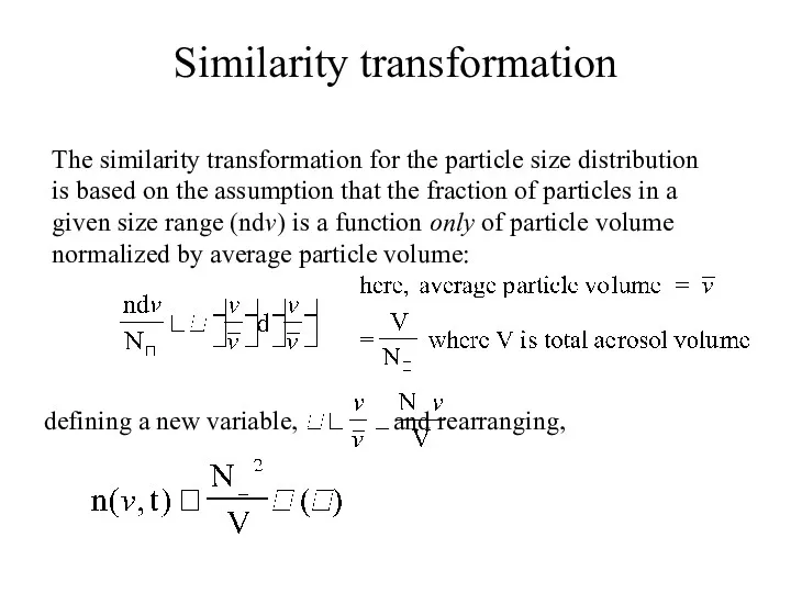
Similarity transformation
The similarity transformation for the particle size distribution
is based on
Similarity transformation
The similarity transformation for the particle size distribution
is based on
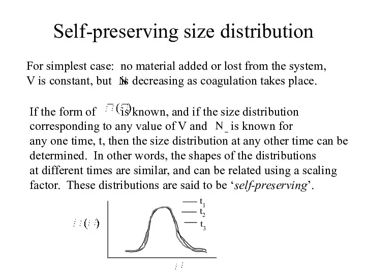
Self-preserving size distribution
For simplest case: no material added or lost from
Self-preserving size distribution
For simplest case: no material added or lost from
 Природные комплексы. Презентация. 6 класс
 Хронический гастрит
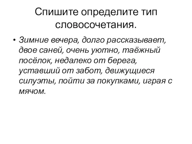 Тип связи в словосочетаниях
 Проект по экспериментальной деятельности Волшебные кристаллы
 Непрерывные сигналы. (Лекция 1.4)
 Влияние цены на излишек производителей
 Эпоха дворцовых переворотов
 Науково-методичні засади організації роботи з обдарованими дітьми
 Аргентина. Визитная карточка
 Презентация Малая летняя академия
 Преимущества и выгода продукции Nature’s Sunshine перед аптечными аналогами
 Информационные жанры. Как писать заметку
 Поздравляем с 23 февраля
 Воспитательный потенциал современной семьи
 Площади подобных фигур
 Вентиляция помещений
 Презентация Шоколад
 Международный день охраны памятников и исторических мест
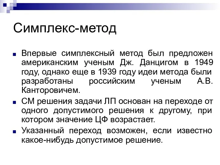 Симплекс-метод
 содержание работы по развитию слухового восприятия речи
 Внеурочная деятельность Мои первые проекты. тема Декупаж
 Направления реализации Национальной стратегии по обращению с ТКО и ВМР
 2.2. Элементарные действия. Алгоритмические структуры [ТРИК]
 Презентация к занятию по предшкольной подготовке Снеговик - почтовик
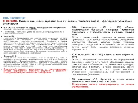 Этнос и этничность в российской этнологии. Признаки этноса – факторы актуализации этничности
 Патофизиология: предмет, задачи, методы
 Ассортимент курток FW 19-20
 Робототехника. Понятие, история и современность