- Real-time PBR Implementation

Содержание
- 2. Image Based Lighting (IBL) Lighting that uses a texture (an image) as light source How is
- 3. Physically Based IBL Ad-hoc IBL vs. Physically-based IBL Has the same differences and similarities between ad-hoc
- 4. Physically Based IBL advantages Guarantees a rendering result that is close to shading under punctual light
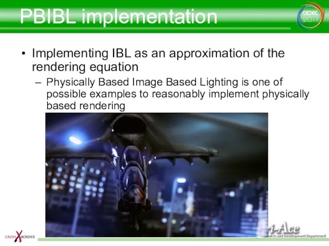
- 5. PBIBL implementation Implementing IBL as an approximation of the rendering equation Physically Based Image Based Lighting
- 6. Equations substitute
- 7. Decompose integral Irradiance Environment Map (IEM) Pre-filtered Radiance Environment Map (PFREM) AmbientBRDF Volume Texture
- 8. Implement Ambient BRDF Precompute this equation off line and store result to a volume texture U
- 9. AmbientBRDF texture usage Fetch the texture For specular component Use the value for For diffuse component
- 10. AmbientBRDF comparison AmbientBRDF OFF AmbientBRDF ON
- 11. Generate textures Use AMD CubeMapGen? It can't be used for real-time processing on multi-platform, because it
- 12. Generate textures Use AMD CubeMapGen? It can't be used for real-time processing on multi-platform, because it
- 13. Generate IEM Implement this equation straightforwardly on GPU Diffuse BRDF is Lambert In the case of
- 14. Generate IEM (2) Using a radiance map reduced to 8x8x6 Store accurately precomputed Δω to the
- 15. Optimize diffuse term Using SH lighting instead of IEM for a high performance configuration Our engine
- 16. Generate REM Pre-filtered Mipmapped Environment Map Compute the equation with different shininess values and store results
- 17. Fitting shininess shininess = 5 shininess =100
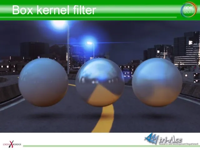
- 18. Generate PMREM (1) Box-filter kernel filtering Simply use bilinear filtering to generate mipmaps LOD values are
- 19. Box kernel filter
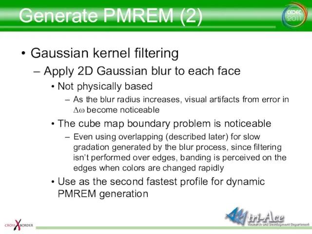
- 20. Generate PMREM (2) Gaussian kernel filtering Apply 2D Gaussian blur to each face Not physically based
- 21. Gaussian kernel filter
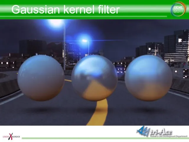
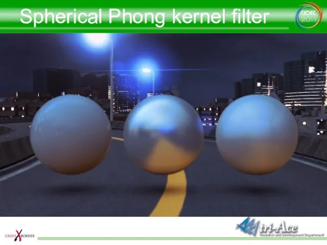
- 22. Generate PMREM(3) Spherical Phong kernel filtering The shininess values are converted using the fitting function The
- 23. Spherical Phong kernel filter
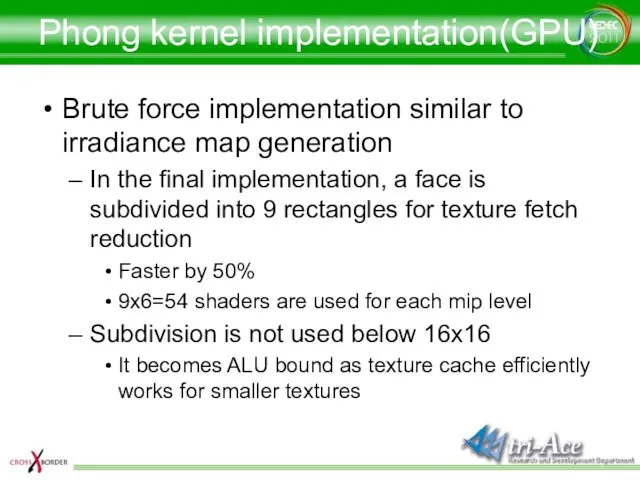
- 24. Phong kernel implementation(GPU) Brute force implementation similar to irradiance map generation In the final implementation, a
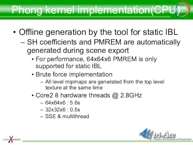
- 25. Phong kernel implementation(CPU) Offline generation by the tool for static IBL SH coefficients and PMREM are
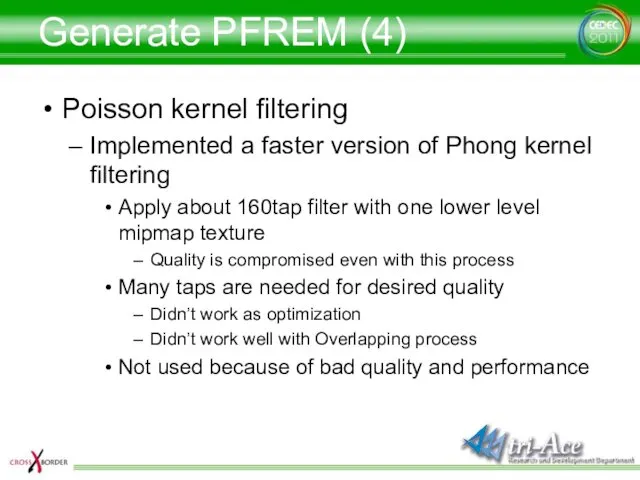
- 26. Generate PFREM (4) Poisson kernel filtering Implemented a faster version of Phong kernel filtering Apply about
- 27. Comparisons Box kernel filter Gaussian kernel filter Spherical Phong kernel filter Spherical Phong kernel filter
- 28. Mipmap LOD Mipmap LOD parameter is calculated for generated PMREM Select the mip level according to
- 29. Edge overlapping Need to solve the cubemap boundary problem No bilinear filtering is applied on the
- 30. Edge overlapping (1) Blend adjacent boundaries by 50% Simplified version of AMD CubeMapGen’s Edge Fixup Adjacent
- 31. Edge overlapping (1)
- 32. Edge overlapping (2) Blend multiple texels For the next step, blend 2 texels In order to
- 33. Edge overlapping (3) 4 texel blend? More blends don’t make sense according to our research 4
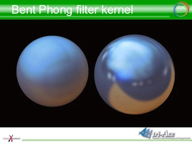
- 34. Bent Phong filter kernel This algorithm blends normals instead of colors Similar to the difference between
- 35. Bent Phong filter kernel
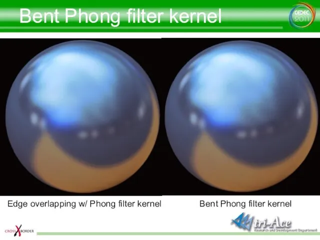
- 36. Bent Phong filter kernel Bent Phong filter kernel Edge overlapping w/ Phong filter kernel
- 37. Implemented configurations Dynamic IBL Static IBL
- 38. Problems with large shininess In practice with IBL, materials still look glossy even with shininess of
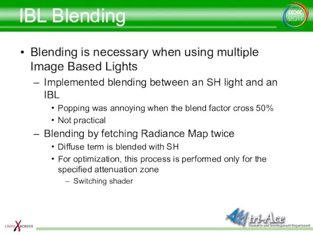
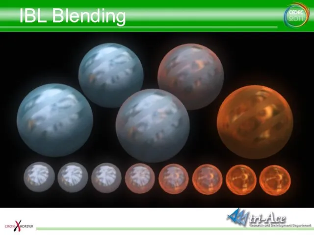
- 39. IBL Blending Blending is necessary when using multiple Image Based Lights Implemented blending between an SH
- 40. IBL Blending
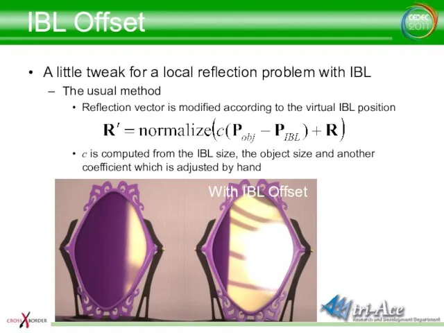
- 41. IBL Offset A little tweak for a local reflection problem with IBL The usual method Reflection
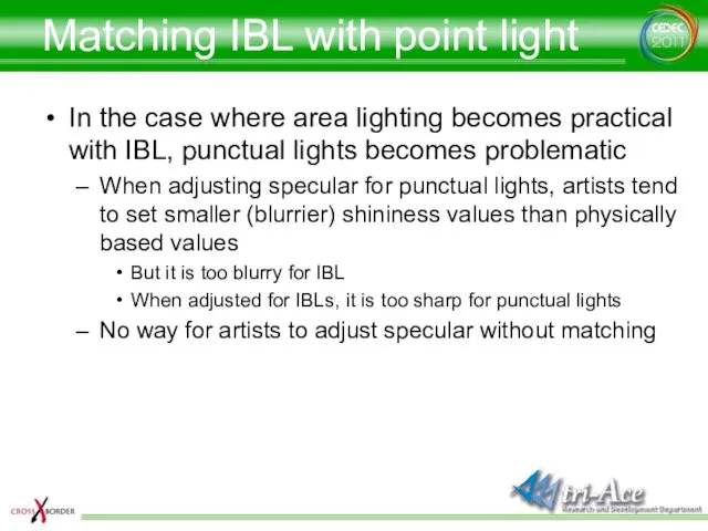
- 42. Matching IBL with point light In the case where area lighting becomes practical with IBL, punctual
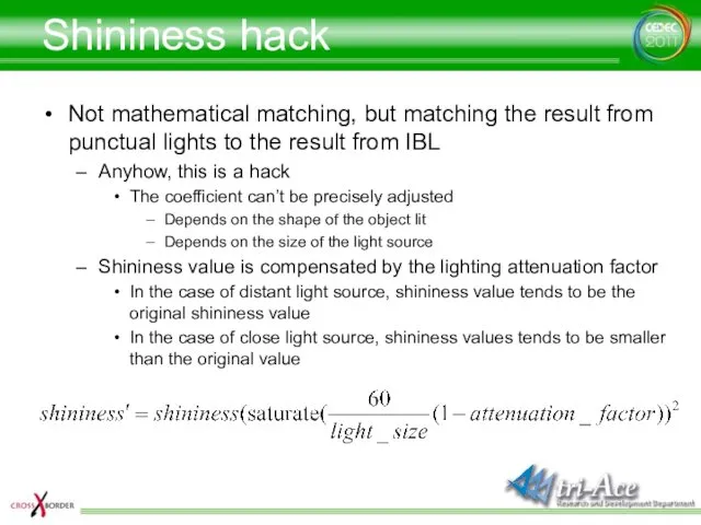
- 43. Shininess hack Not mathematical matching, but matching the result from punctual lights to the result from
- 44. Shininess hack
- 45. Shininess hack
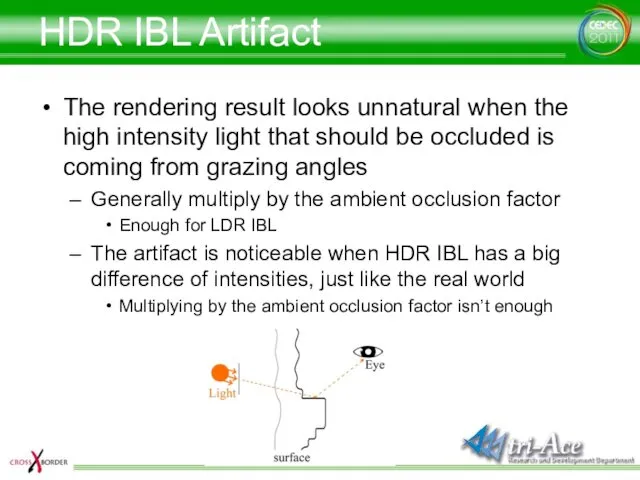
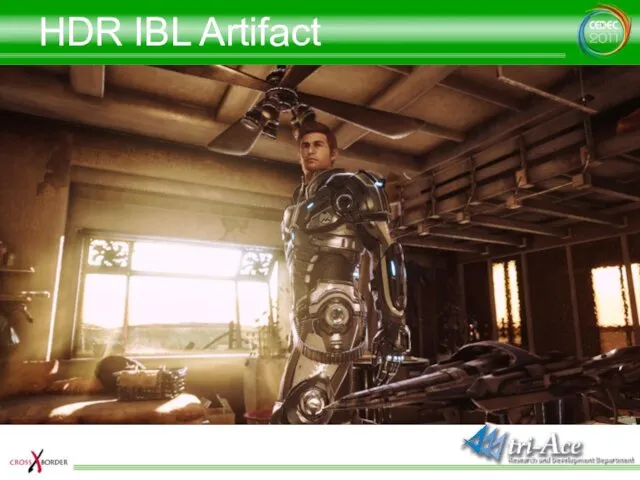
- 46. HDR IBL Artifact The rendering result looks unnatural when the high intensity light that should be
- 47. HDR IBL Artifact
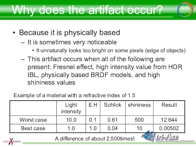
- 48. Why does the artifact occur? Because it is physically based It is sometimes very noticeable It
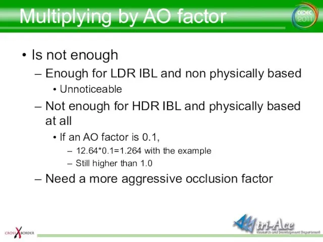
- 49. Multiplying by AO factor Is not enough Enough for LDR IBL and non physically based Unnoticeable
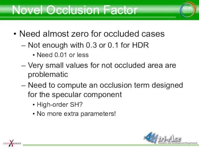
- 50. Novel Occlusion Factor Need almost zero for occluded cases Not enough with 0.3 or 0.1 for
- 51. Specular Occlusion SO is acquired from AO Use AO factor as HBAO or SSAO But precomputed
- 52. Aqcuire Specular Occlusion In the case where a pixel is isotropically occluded from the horizon without
- 53. Specular Occlusion implementation Required SO (Specular Occlusion) factor should satisfy the following as much as possible
- 54. Specular Occlusion Ambient Occlusion Specular Occlusion
- 55. SO implementation (1) The first equation that satisfies the condition Though this satisfies the conditions as
- 56. SO implementation (1)
- 57. SO implementation (2) Equation taking into account the shininess value More physically based than the first
- 58. SO implementation (2)
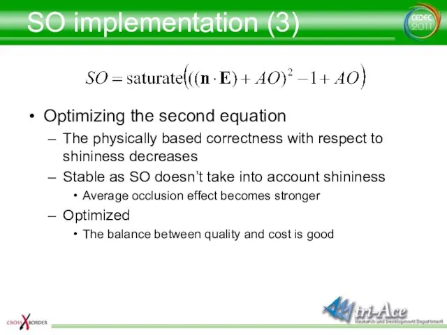
- 59. SO implementation (3) Optimizing the second equation The physically based correctness with respect to shininess decreases
- 60. SO implementation (3)
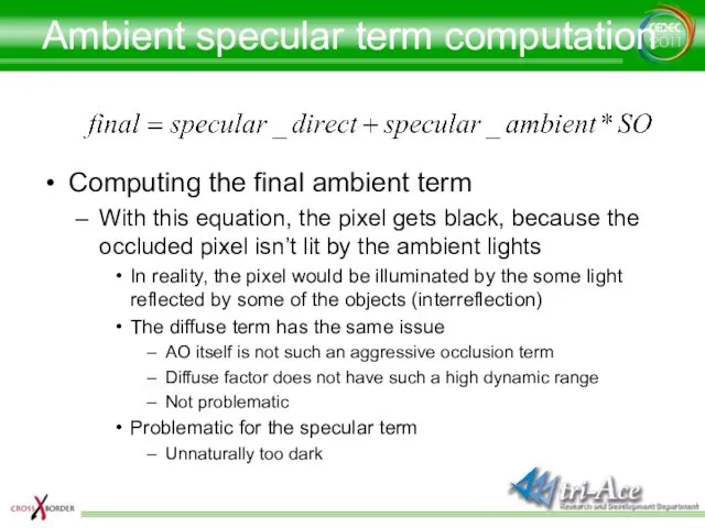
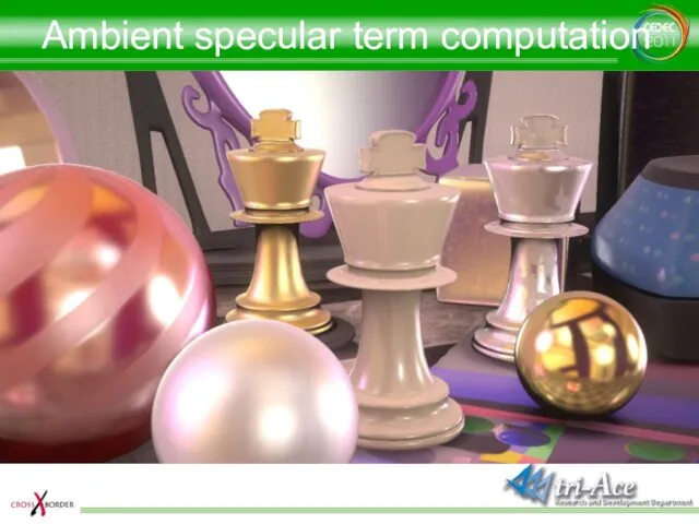
- 61. Ambient specular term computation Computing the final ambient term With this equation, the pixel gets black,
- 62. Ambient specular term computation
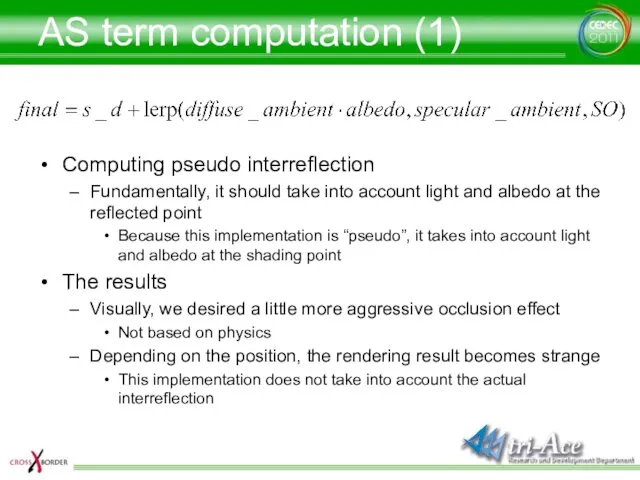
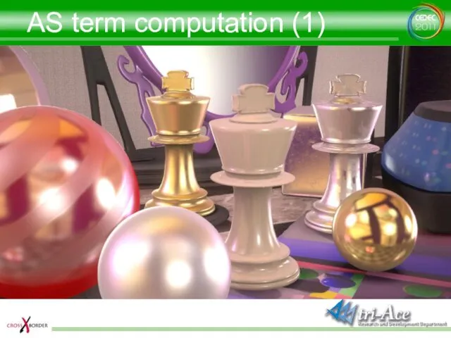
- 63. AS term computation (1) Computing pseudo interreflection Fundamentally, it should take into account light and albedo
- 64. AS term computation (1)
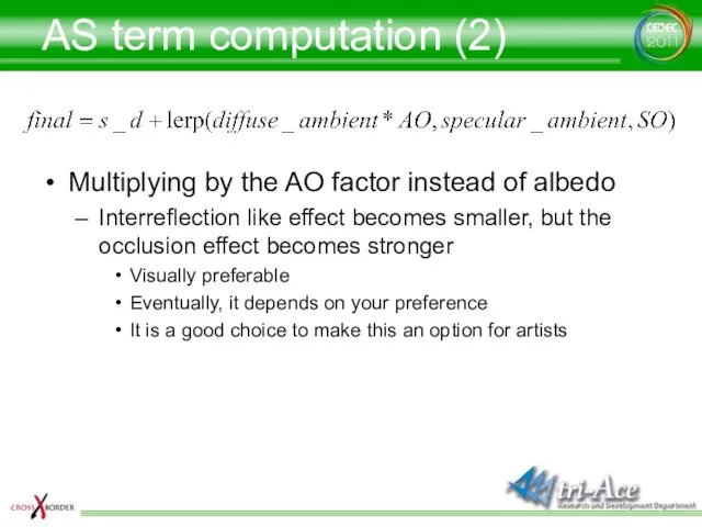
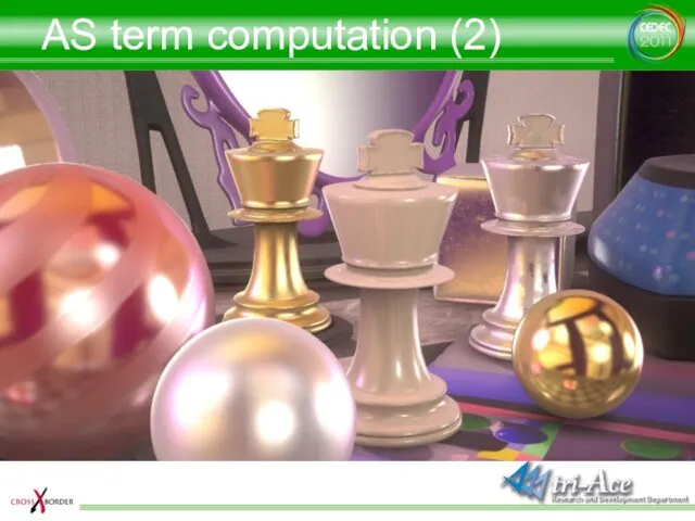
- 65. AS term computation (2) Multiplying by the AO factor instead of albedo Interreflection like effect becomes
- 66. AS term computation (2)
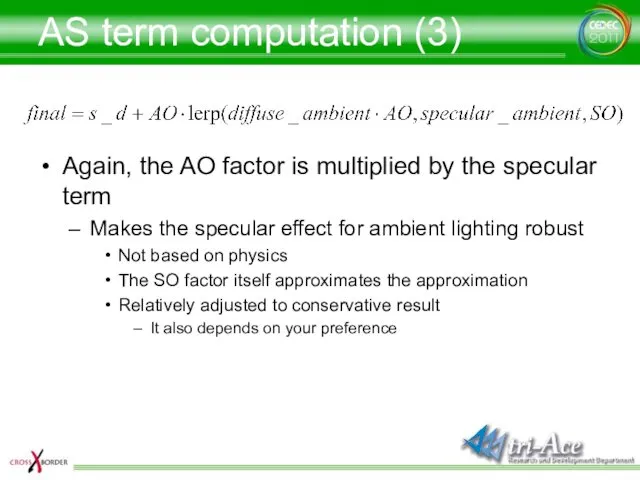
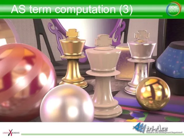
- 67. AS term computation (3) Again, the AO factor is multiplied by the specular term Makes the
- 68. AS term computation (3)
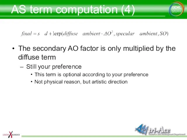
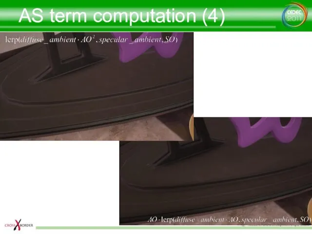
- 69. AS term computation (4) The secondary AO factor is only multiplied by the diffuse term Still
- 70. AS term computation (4)
- 71. Applying to the entire specular term SO factor is also available for the specular term with
- 72. W/o Specular Occlusion (Only AO)
- 73. With Specular Occlusion
- 74. IBL performance ms @ 1280x720
- 75. Physically based IBL
- 76. Physically based IBL
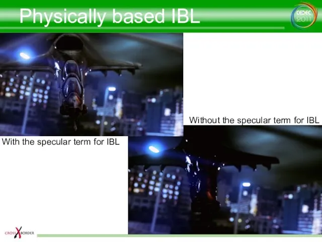
- 77. Physically based IBL With the specular term for IBL Without the specular term for IBL
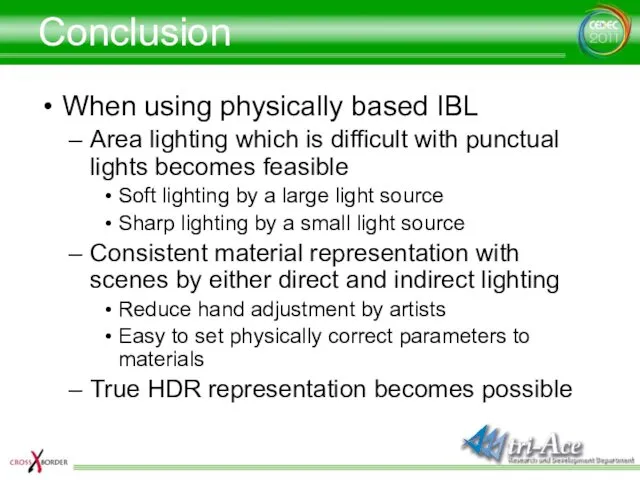
- 78. Conclusion When using physically based IBL Area lighting which is difficult with punctual lights becomes feasible
- 79. Acknowledgements R&D department, tri-Ace, Inc. Tatsuya Shoji Elliott Davis Thanks for the English version Sébastien Lagarde,
- 81. Скачать презентацию
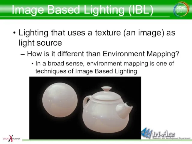
Image Based Lighting (IBL)
Lighting that uses a texture (an image) as
Image Based Lighting (IBL)
Lighting that uses a texture (an image) as
Physically Based IBL
Ad-hoc IBL vs. Physically-based IBL
Has the same differences and
Physically Based IBL
Ad-hoc IBL vs. Physically-based IBL
Has the same differences and
Physically Based IBL advantages
Guarantees a rendering result that is close to
Physically Based IBL advantages
Guarantees a rendering result that is close to
PBIBL implementation
Implementing IBL as an approximation of the rendering equation
Physically Based
PBIBL implementation
Implementing IBL as an approximation of the rendering equation
Physically Based
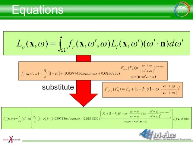
Equations
substitute
Equations
substitute
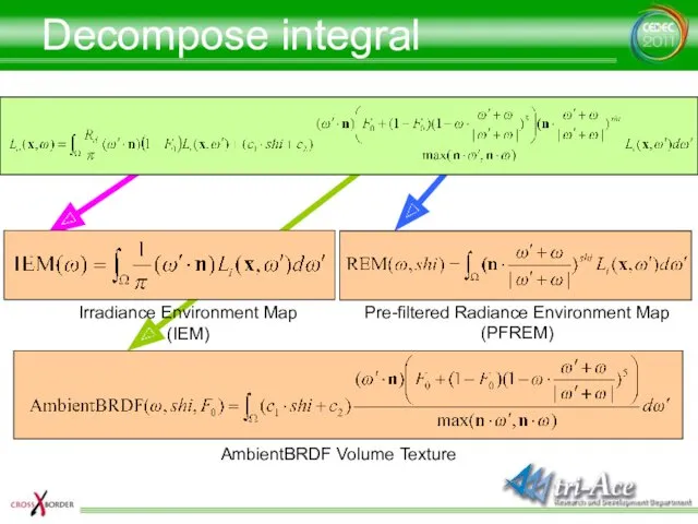
Decompose integral
Irradiance Environment Map (IEM)
Pre-filtered Radiance Environment Map
(PFREM)
AmbientBRDF Volume Texture
Decompose integral
Irradiance Environment Map (IEM)
Pre-filtered Radiance Environment Map
(PFREM)
AmbientBRDF Volume Texture
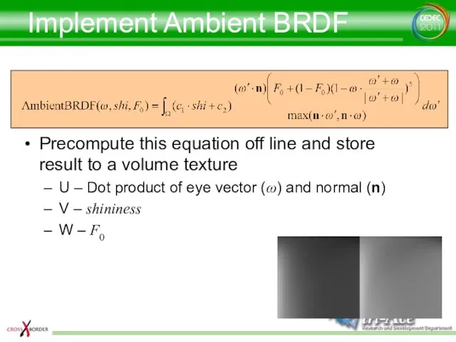
Implement Ambient BRDF
Precompute this equation off line and store result to
Implement Ambient BRDF
Precompute this equation off line and store result to
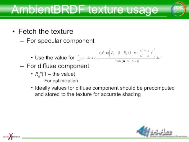
AmbientBRDF texture usage
Fetch the texture
For specular component
Use the value for
For diffuse
AmbientBRDF texture usage
Fetch the texture
For specular component
Use the value for
For diffuse
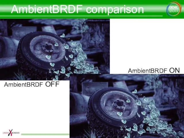
AmbientBRDF comparison
AmbientBRDF OFF
AmbientBRDF ON
AmbientBRDF comparison
AmbientBRDF OFF
AmbientBRDF ON

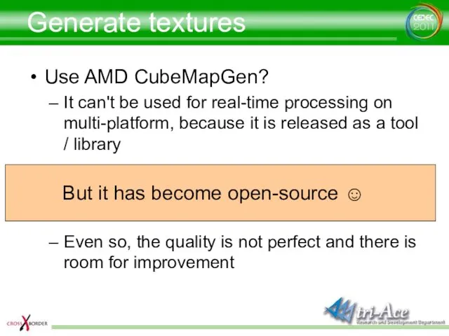
Generate textures
Use AMD CubeMapGen?
It can't be used for real-time processing on
Generate textures
Use AMD CubeMapGen?
It can't be used for real-time processing on
Generate textures
Use AMD CubeMapGen?
It can't be used for real-time processing on
Generate textures
Use AMD CubeMapGen?
It can't be used for real-time processing on
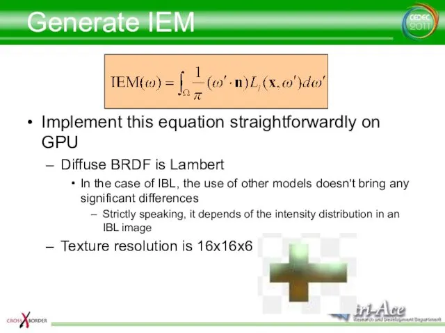
Generate IEM
Implement this equation straightforwardly on GPU
Diffuse BRDF is Lambert
In the
Generate IEM
Implement this equation straightforwardly on GPU
Diffuse BRDF is Lambert
In the
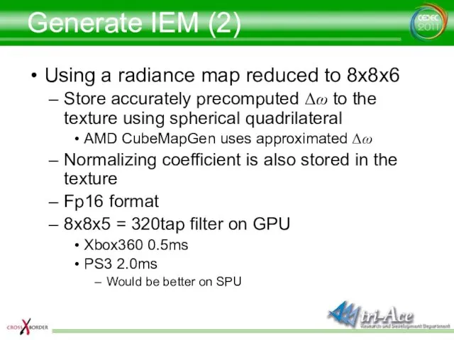
Generate IEM (2)
Using a radiance map reduced to 8x8x6
Store accurately precomputed
Generate IEM (2)
Using a radiance map reduced to 8x8x6
Store accurately precomputed
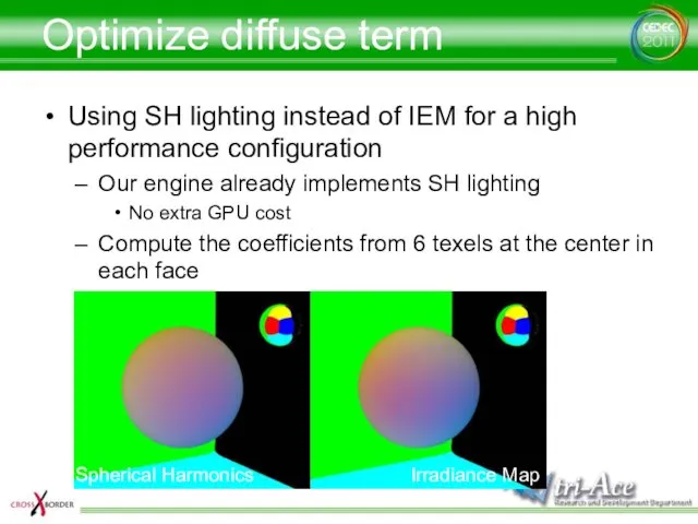
Optimize diffuse term
Using SH lighting instead of IEM for a high
Optimize diffuse term
Using SH lighting instead of IEM for a high
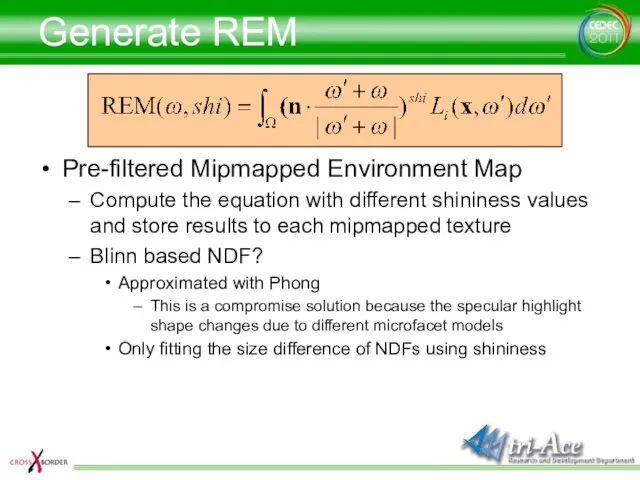
Generate REM
Pre-filtered Mipmapped Environment Map
Compute the equation with different shininess values
Generate REM
Pre-filtered Mipmapped Environment Map
Compute the equation with different shininess values
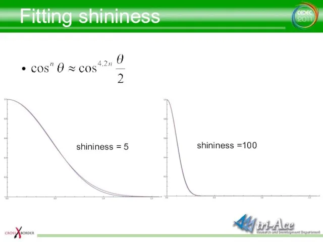
Fitting shininess
shininess = 5
shininess =100
Fitting shininess
shininess = 5
shininess =100
Generate PMREM (1)
Box-filter kernel filtering
Simply use bilinear filtering to generate mipmaps
LOD
Generate PMREM (1)
Box-filter kernel filtering
Simply use bilinear filtering to generate mipmaps
LOD
Box kernel filter
Box kernel filter
Generate PMREM (2)
Gaussian kernel filtering
Apply 2D Gaussian blur to each face
Not
Generate PMREM (2)
Gaussian kernel filtering
Apply 2D Gaussian blur to each face
Not
Gaussian kernel filter
Gaussian kernel filter
Generate PMREM(3)
Spherical Phong kernel filtering
The shininess values are converted using the
Generate PMREM(3)
Spherical Phong kernel filtering
The shininess values are converted using the
Spherical Phong kernel filter
Spherical Phong kernel filter
Phong kernel implementation(GPU)
Brute force implementation similar to irradiance map generation
In the
Phong kernel implementation(GPU)
Brute force implementation similar to irradiance map generation
In the
Phong kernel implementation(CPU)
Offline generation by the tool for static IBL
SH coefficients
Phong kernel implementation(CPU)
Offline generation by the tool for static IBL
SH coefficients
Generate PFREM (4)
Poisson kernel filtering
Implemented a faster version of Phong kernel
Generate PFREM (4)
Poisson kernel filtering
Implemented a faster version of Phong kernel
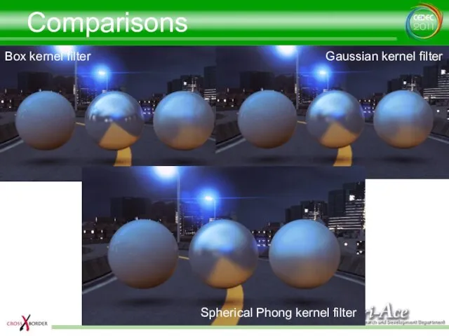
Comparisons
Box kernel filter
Gaussian kernel filter
Spherical Phong kernel filter
Spherical Phong kernel filter
Comparisons
Box kernel filter
Gaussian kernel filter
Spherical Phong kernel filter
Spherical Phong kernel filter
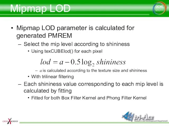
Mipmap LOD
Mipmap LOD parameter is calculated for generated PMREM
Select the mip
Mipmap LOD
Mipmap LOD parameter is calculated for generated PMREM
Select the mip
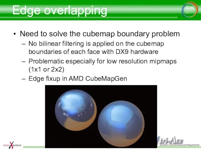
Edge overlapping
Need to solve the cubemap boundary problem
No bilinear filtering is
Edge overlapping
Need to solve the cubemap boundary problem
No bilinear filtering is
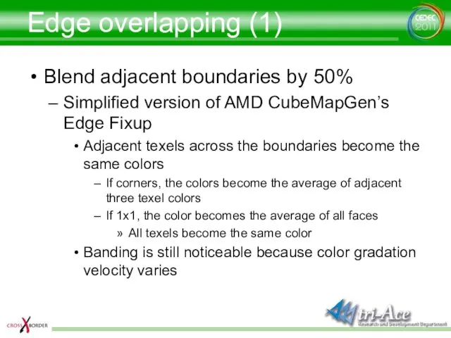
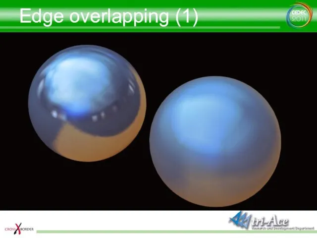
Edge overlapping (1)
Blend adjacent boundaries by 50%
Simplified version of AMD CubeMapGen’s
Edge overlapping (1)
Blend adjacent boundaries by 50%
Simplified version of AMD CubeMapGen’s
Edge overlapping (1)
Edge overlapping (1)
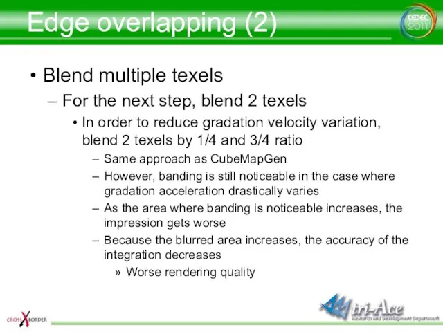
Edge overlapping (2)
Blend multiple texels
For the next step, blend 2 texels
In
Edge overlapping (2)
Blend multiple texels
For the next step, blend 2 texels
In
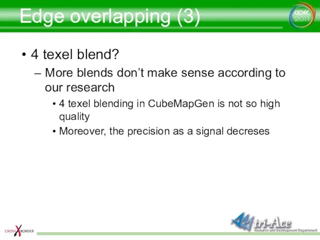
Edge overlapping (3)
4 texel blend?
More blends don’t make sense according to
Edge overlapping (3)
4 texel blend?
More blends don’t make sense according to
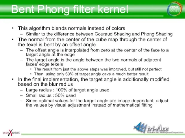
Bent Phong filter kernel
This algorithm blends normals instead of colors
Similar to
Bent Phong filter kernel
This algorithm blends normals instead of colors
Similar to
Bent Phong filter kernel
Bent Phong filter kernel
Bent Phong filter kernel
Bent Phong filter kernel
Edge overlapping w/ Phong filter
Bent Phong filter kernel
Bent Phong filter kernel
Edge overlapping w/ Phong filter
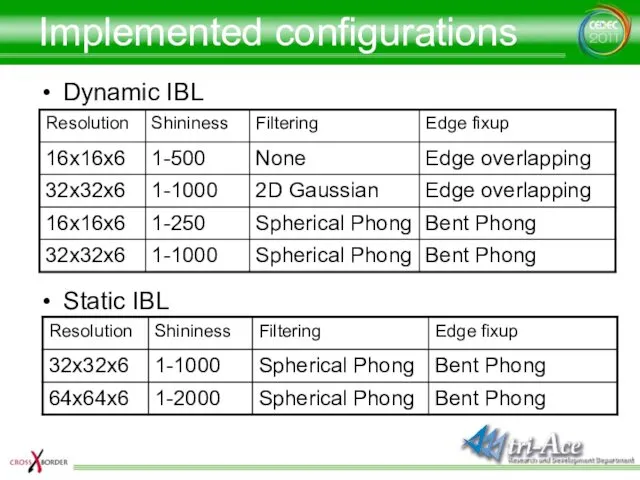
Implemented configurations
Dynamic IBL
Static IBL
Implemented configurations
Dynamic IBL
Static IBL
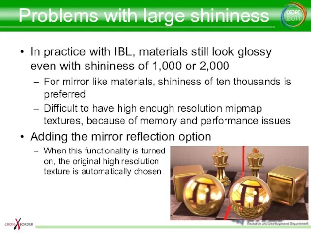
Problems with large shininess
In practice with IBL, materials still look glossy
Problems with large shininess
In practice with IBL, materials still look glossy
IBL Blending
Blending is necessary when using multiple Image Based Lights
Implemented blending
IBL Blending
Blending is necessary when using multiple Image Based Lights
Implemented blending
IBL Blending
IBL Blending
IBL Offset
A little tweak for a local reflection problem with IBL
The
IBL Offset
A little tweak for a local reflection problem with IBL
The
Matching IBL with point light
In the case where area lighting becomes
Matching IBL with point light
In the case where area lighting becomes
Shininess hack
Not mathematical matching, but matching the result from punctual lights
Shininess hack
Not mathematical matching, but matching the result from punctual lights
Shininess hack
Shininess hack
Shininess hack
Shininess hack
HDR IBL Artifact
The rendering result looks unnatural when the high intensity
HDR IBL Artifact
The rendering result looks unnatural when the high intensity
HDR IBL Artifact
HDR IBL Artifact
Why does the artifact occur?
Because it is physically based
It is sometimes
Why does the artifact occur?
Because it is physically based
It is sometimes
Multiplying by AO factor
Is not enough
Enough for LDR IBL and non
Multiplying by AO factor
Is not enough
Enough for LDR IBL and non
Novel Occlusion Factor
Need almost zero for occluded cases
Not enough with 0.3
Novel Occlusion Factor
Need almost zero for occluded cases
Not enough with 0.3
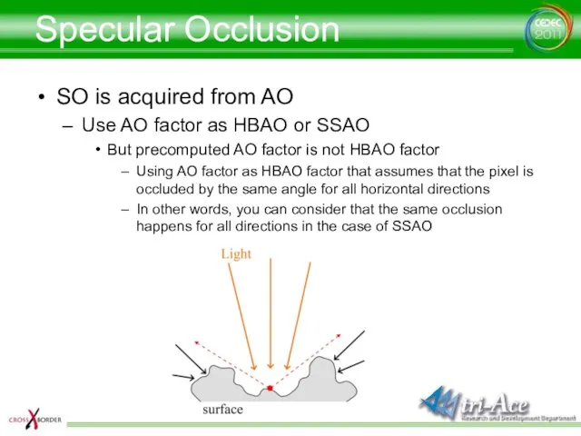
Specular Occlusion
SO is acquired from AO
Use AO factor as HBAO or
Specular Occlusion
SO is acquired from AO
Use AO factor as HBAO or
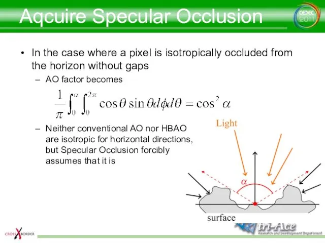
Aqcuire Specular Occlusion
In the case where a pixel is isotropically occluded
Aqcuire Specular Occlusion
In the case where a pixel is isotropically occluded
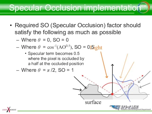
Specular Occlusion implementation
Required SO (Specular Occlusion) factor should satisfy the following
Specular Occlusion implementation
Required SO (Specular Occlusion) factor should satisfy the following
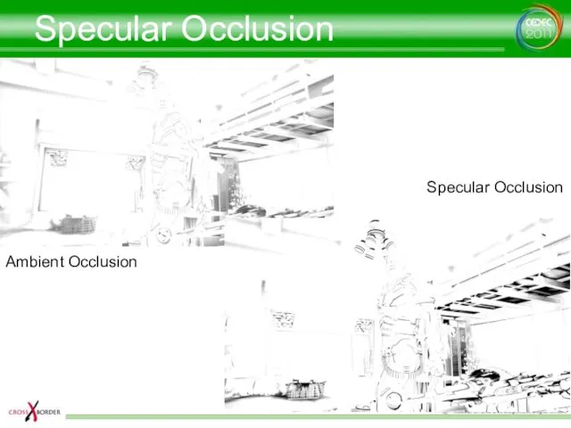
Specular Occlusion
Ambient Occlusion
Specular Occlusion
Specular Occlusion
Ambient Occlusion
Specular Occlusion
SO implementation (1)
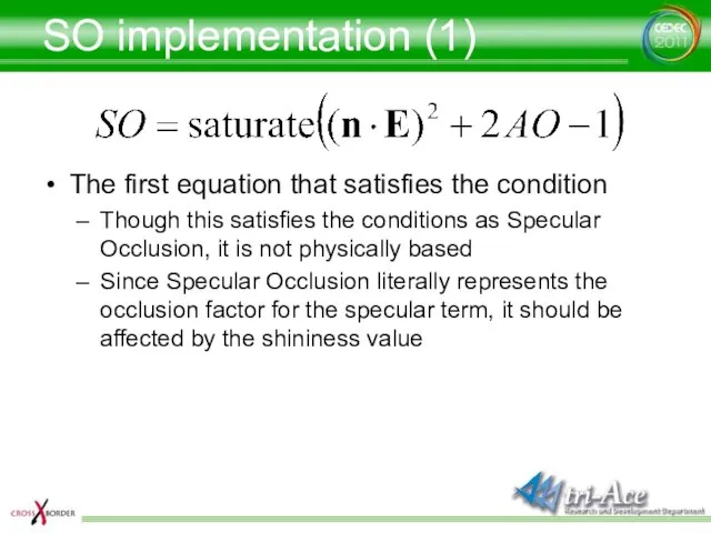
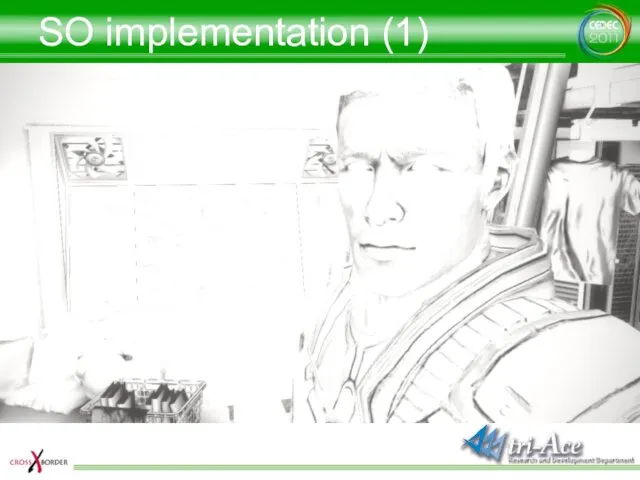
The first equation that satisfies the condition
Though this satisfies
SO implementation (1)
The first equation that satisfies the condition
Though this satisfies
SO implementation (1)
SO implementation (1)
SO implementation (2)
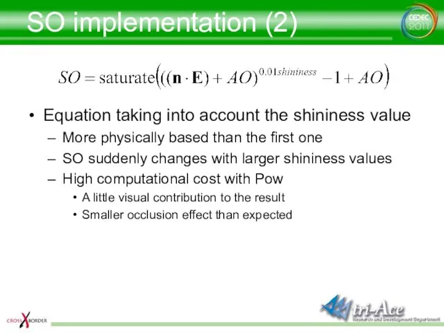
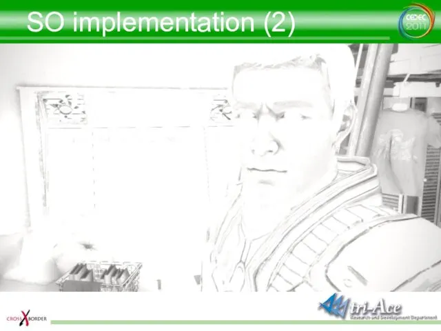
Equation taking into account the shininess value
More physically based
SO implementation (2)
Equation taking into account the shininess value
More physically based
SO implementation (2)
SO implementation (2)
SO implementation (3)
Optimizing the second equation
The physically based correctness with respect
SO implementation (3)
Optimizing the second equation
The physically based correctness with respect
SO implementation (3)
SO implementation (3)
Ambient specular term computation
Computing the final ambient term
With this equation, the
Ambient specular term computation
Computing the final ambient term
With this equation, the
Ambient specular term computation
Ambient specular term computation
AS term computation (1)
Computing pseudo interreflection
Fundamentally, it should take into account
AS term computation (1)
Computing pseudo interreflection
Fundamentally, it should take into account
AS term computation (1)
AS term computation (1)
AS term computation (2)
Multiplying by the AO factor instead of albedo
Interreflection
AS term computation (2)
Multiplying by the AO factor instead of albedo
Interreflection
AS term computation (2)
AS term computation (2)
AS term computation (3)
Again, the AO factor is multiplied by the
AS term computation (3)
Again, the AO factor is multiplied by the
AS term computation (3)
AS term computation (3)
AS term computation (4)
The secondary AO factor is only multiplied by
AS term computation (4)
The secondary AO factor is only multiplied by
AS term computation (4)
AS term computation (4)
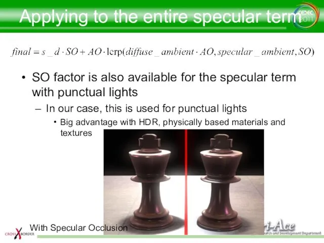
Applying to the entire specular term
SO factor is also available for
Applying to the entire specular term
SO factor is also available for
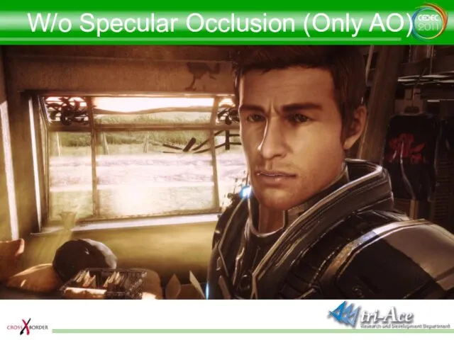
W/o Specular Occlusion (Only AO)
W/o Specular Occlusion (Only AO)
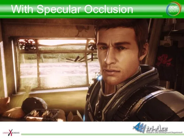
With Specular Occlusion
With Specular Occlusion
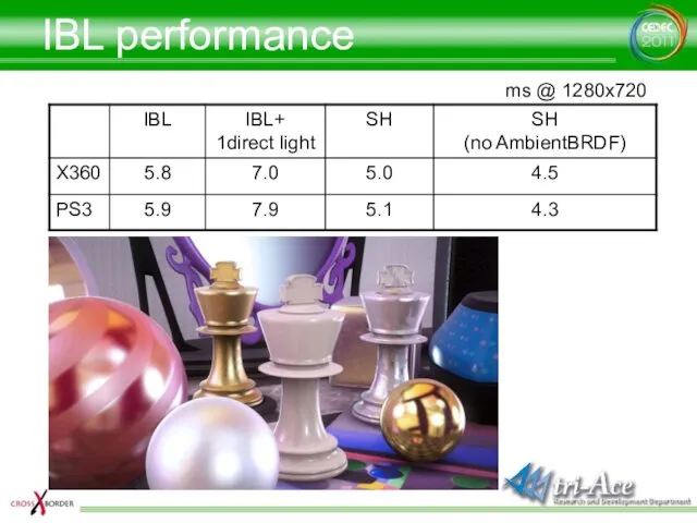
IBL performance
ms @ 1280x720
IBL performance
ms @ 1280x720
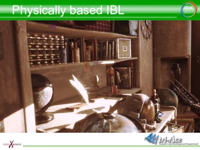
Physically based IBL
Physically based IBL
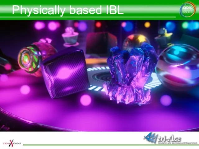
Physically based IBL
Physically based IBL
Physically based IBL
With the specular term for IBL
Without the specular term
Physically based IBL
With the specular term for IBL
Without the specular term
Conclusion
When using physically based IBL
Area lighting which is difficult with punctual
Conclusion
When using physically based IBL
Area lighting which is difficult with punctual
Acknowledgements
R&D department, tri-Ace, Inc.
Tatsuya Shoji
Elliott Davis
Thanks for the English version
Sébastien Lagarde,
Acknowledgements
R&D department, tri-Ace, Inc.
Tatsuya Shoji
Elliott Davis
Thanks for the English version
Sébastien Lagarde,
 Плавание. Общий курс
 Создание и анализ данных в современных СУБД
 Н. Сладков. Лисица и Ёж
 Гетьман Конашевич-Сагайдачний
 Построение двойственной задачи
 Бабочка из бумаги (1 класс)
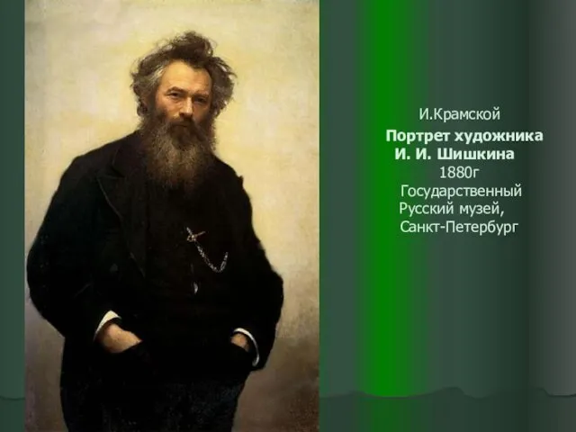 Картины И.И. Шишкина
 Функциональные системы автоматизации технологических процессов. Автоматизация добычи промыслового сбора нефти и нефтяного газа
 Принципы взаимодействия с родителями
 презентация Ионные уравнения
 Проектная работа География на подоконнике
 Адаптация – результат эволюции
 Социальные статусы и роли
 Урок знаний
 Система ремонта техники связи и АСУ (лекции № 7)
 2 курс Культура речи 3, 4
 Человек, как духовное существо
 Мастер-класс для педагогов. Интеллектуальная игра Мозговой штурм
 Презентация для старших дошкольников Успение Пресвятой Богородицы
 Мастер-класс по химии Расстановка коэффициентов в химических уравнениях
 Страшилки. Не трогай старый сундук
 Волшебные свойства бумаги
 Балада про цибулю
 Биохимия крови
 Л 1 Числ множ Предел последов
 Прямая и обратная теоремы Виета
 Цивилизации Запада и Востока в Средние века. Варварские государства. Раннее средневековье в Европе
 Efes Manufacturing System