- Solution methods for bilevel optimization

Содержание
- 2. Overview Definition of a bilevel problem and its general form Optimality (KKT-type) conditions Reformulation of a
- 3. Stackelberg Game (Bilevel problem) Players: the Leader and the Follower The Leader is first to make
- 4. Example Taxation of a factory Leader – government Objectives: maximize profit and minimize pollution Follower –
- 5. General structure of a Bilevel problem
- 6. Important Sets
- 7. General linear Bilevel problem
- 8. Solution methods Vertex enumeration in the context of Simplex method Kuhn-Tucker approach Penalty approach Extract gradient
- 9. Concept of KKT conditions
- 10. Value function reformulation
- 11. KKT for value function reformulation
- 12. Assumptions
- 13. KKT-type optimality conditions for Bilevel
- 14. Further Assumptions (for simpler version)
- 15. Simpler version of KKT-type conditions
- 16. NCP-Functions
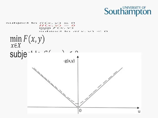
- 17. Problems with differentiability Fischer-Burmeister is not differentiable at 0
- 19. Simpler version with perturbed Fischer-Burmeister NCP functions
- 20. Iterative methods
- 21. Newton method
- 22. Pseudo inverse
- 23. Gauss-Newton method
- 24. Singular Value Decomposition (SVD)
- 25. SVD for wrong direction
- 26. SVD for right direction
- 27. Levenberg-Marquardt method
- 28. Numerical results
- 29. Plans for further work
- 30. Plans for further work 6. Construct the own code for Levenberg-Marquardt method in the context of
- 31. Thank you! Questions?
- 32. References
- 34. Скачать презентацию
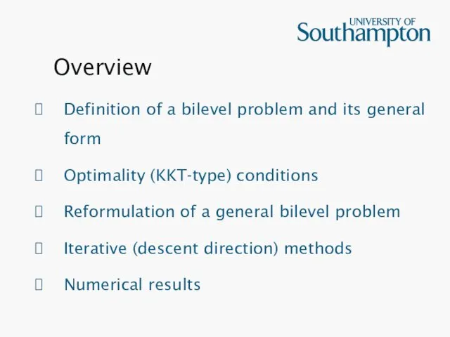
Overview
Definition of a bilevel problem and its general form
Optimality (KKT-type) conditions
Reformulation
Overview
Definition of a bilevel problem and its general form
Optimality (KKT-type) conditions
Reformulation
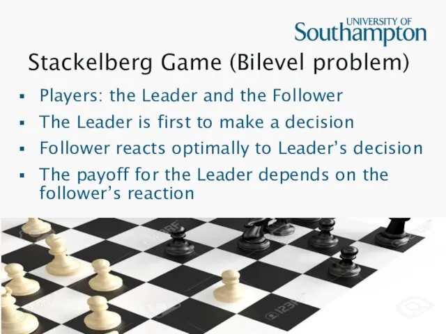
Stackelberg Game (Bilevel problem)
Players: the Leader and the Follower
The Leader is
Stackelberg Game (Bilevel problem)
Players: the Leader and the Follower
The Leader is
Example
Taxation of a factory
Leader – government
Objectives: maximize profit and minimize pollution
Follower
Example
Taxation of a factory
Leader – government
Objectives: maximize profit and minimize pollution
Follower
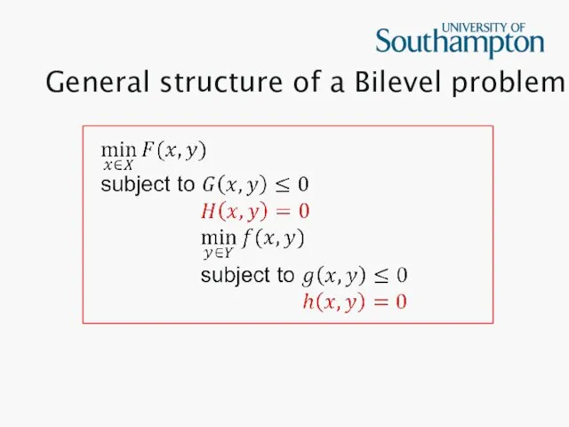
General structure of a Bilevel problem
General structure of a Bilevel problem
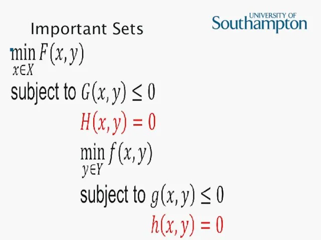
Important Sets
Important Sets
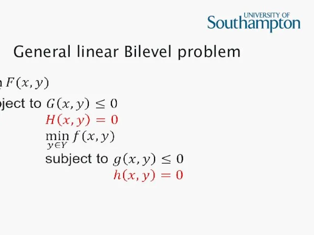
General linear Bilevel problem
General linear Bilevel problem
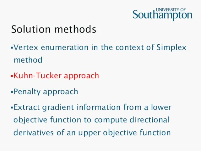
Solution methods
Vertex enumeration in the context of Simplex method
Kuhn-Tucker approach
Penalty approach
Extract
Solution methods
Vertex enumeration in the context of Simplex method
Kuhn-Tucker approach
Penalty approach
Extract
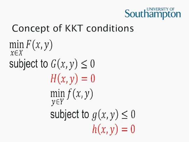
Concept of KKT conditions
Concept of KKT conditions
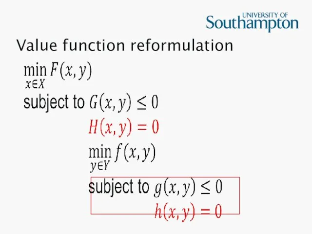
Value function reformulation
Value function reformulation
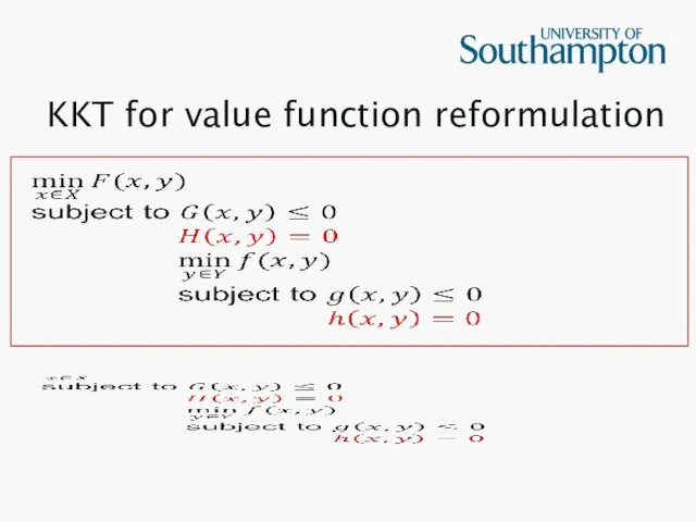
KKT for value function reformulation
KKT for value function reformulation
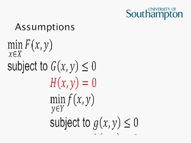
Assumptions
Assumptions
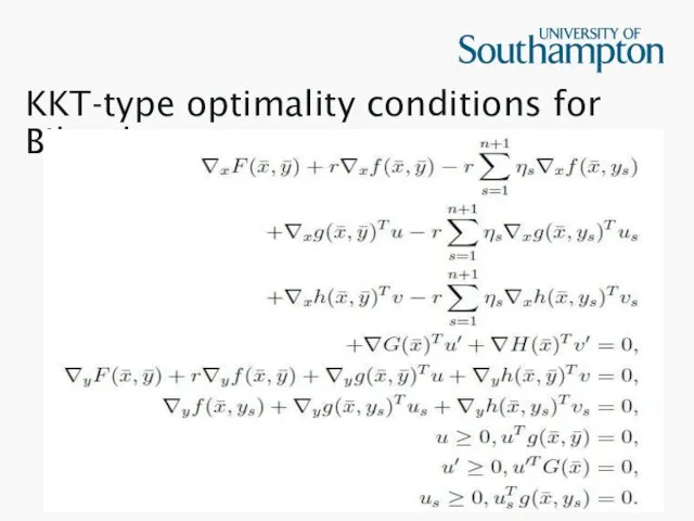
KKT-type optimality conditions for Bilevel
KKT-type optimality conditions for Bilevel
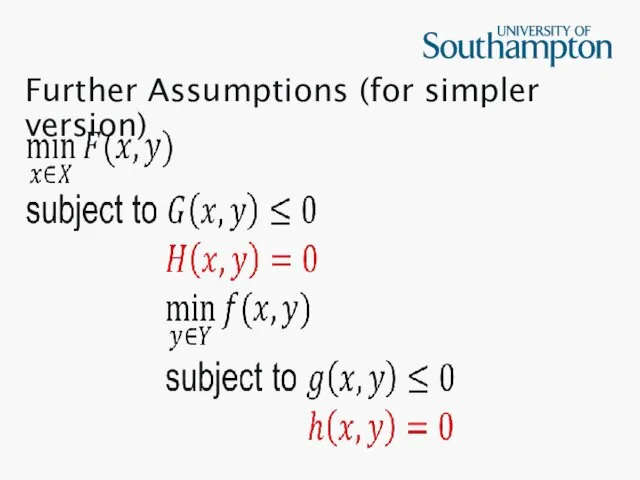
Further Assumptions (for simpler version)
Further Assumptions (for simpler version)
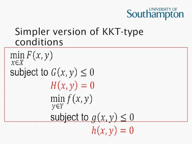
Simpler version of KKT-type conditions
Simpler version of KKT-type conditions
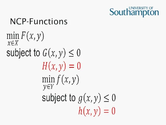
NCP-Functions
NCP-Functions
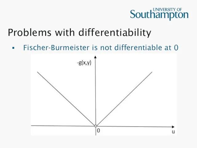
Problems with differentiability
Fischer-Burmeister is not differentiable at 0
Problems with differentiability
Fischer-Burmeister is not differentiable at 0
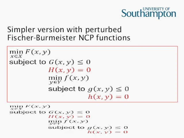
Simpler version with perturbed Fischer-Burmeister NCP functions
Simpler version with perturbed Fischer-Burmeister NCP functions
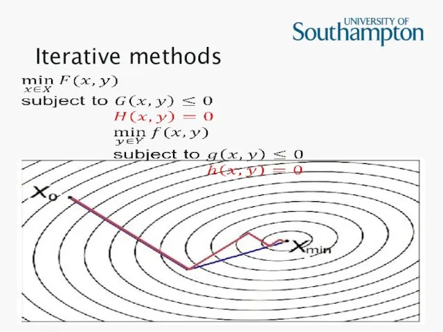
Iterative methods
Iterative methods
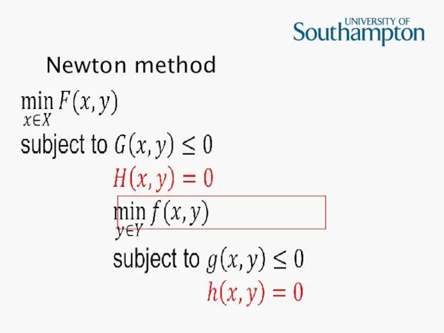
Newton method
Newton method
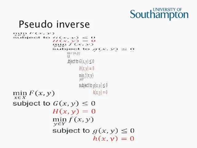
Pseudo inverse
Pseudo inverse
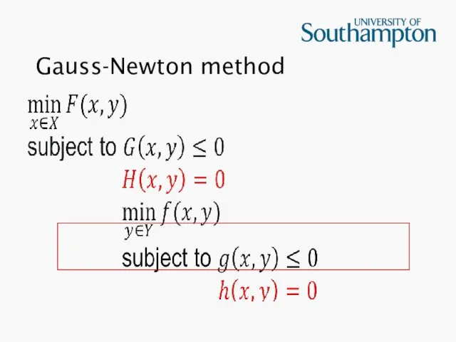
Gauss-Newton method
Gauss-Newton method
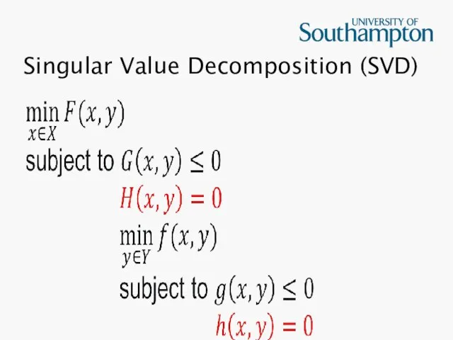
Singular Value Decomposition (SVD)
Singular Value Decomposition (SVD)
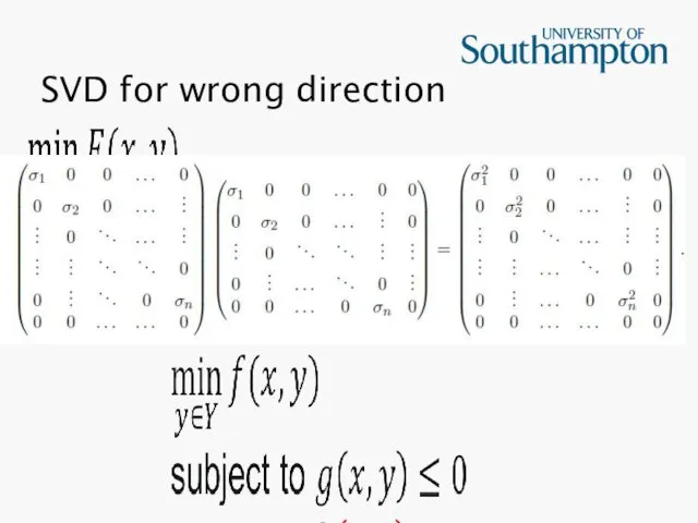
SVD for wrong direction
SVD for wrong direction
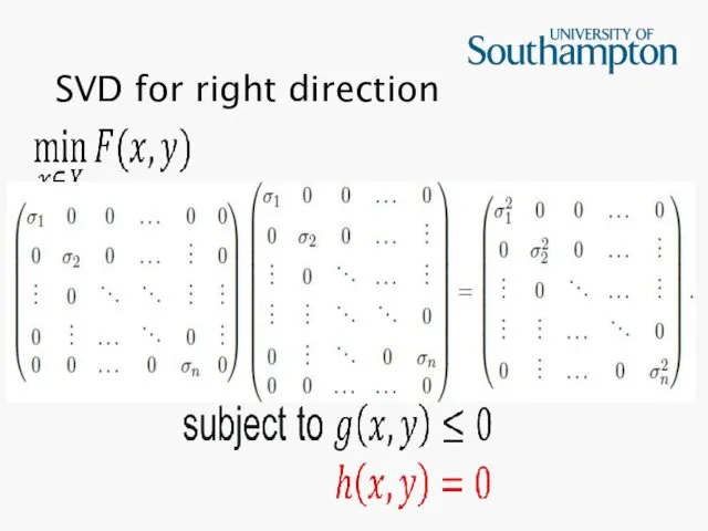
SVD for right direction
SVD for right direction
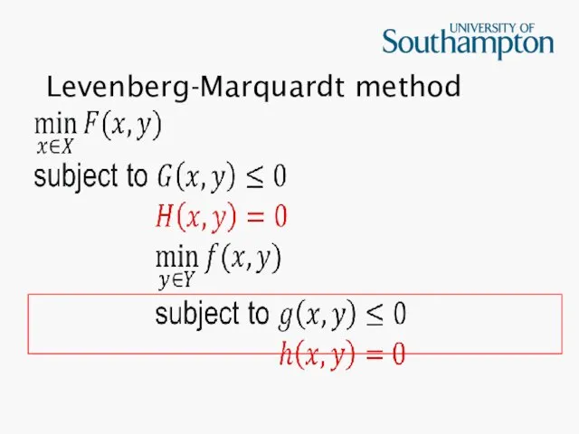
Levenberg-Marquardt method
Levenberg-Marquardt method
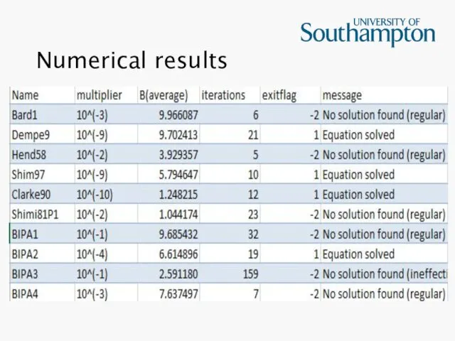
Numerical results
Numerical results

Plans for further work
Plans for further work
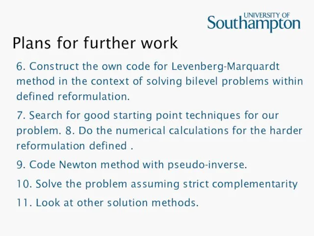
Plans for further work
6. Construct the own code for Levenberg-Marquardt method
Plans for further work
6. Construct the own code for Levenberg-Marquardt method

Thank you!
Questions?
Thank you!
Questions?
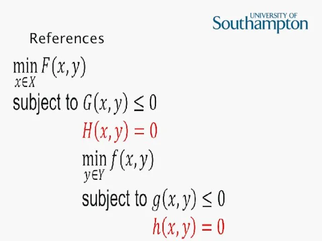
References
References
 Сложноподчиненные предложения
 Методы и методические приемы обучения биологии
 Электродвигатели постоянного тока. Первый этап развития электродвигателя
 Булану мен конденсация
 Дерево тематик. Пассажиры
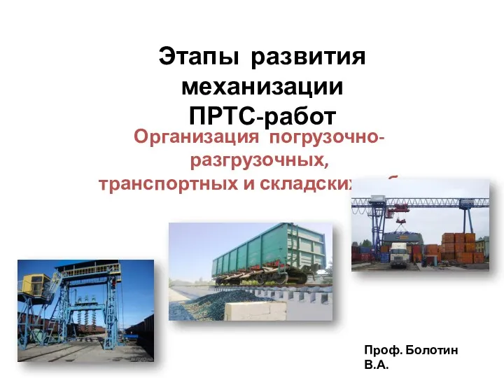 Этапы развития механизации ПРТС-работ. Организация погрузочно-разгрузочных, транспортных и складских работ
 Векторная графика в Web
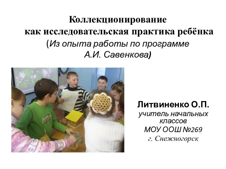 Презентация Коллекционирование как исследовательская практика ребёнка(Из опыта работы по программе А.И. Савенкова)
 деление десятичной дроби на натуральное число
 Типы климатов России разработка урока географии 8 класс
 Всероссийская олимпиада по искусству. Школьный этап. (9-11 класс)
 Рабочий отчет департамента аналитики компании IPO
 There is, are
 Презентация Виды современных велосипедов Диск
 Статистика посещения кинотеатров в России, 2009-2019 годы
 презентация результата совместного проекта с родителями
 Тест. Планеты Солнечной системы
 Презентации по основам православной культуры
 Кодекс этической деятельности педагога
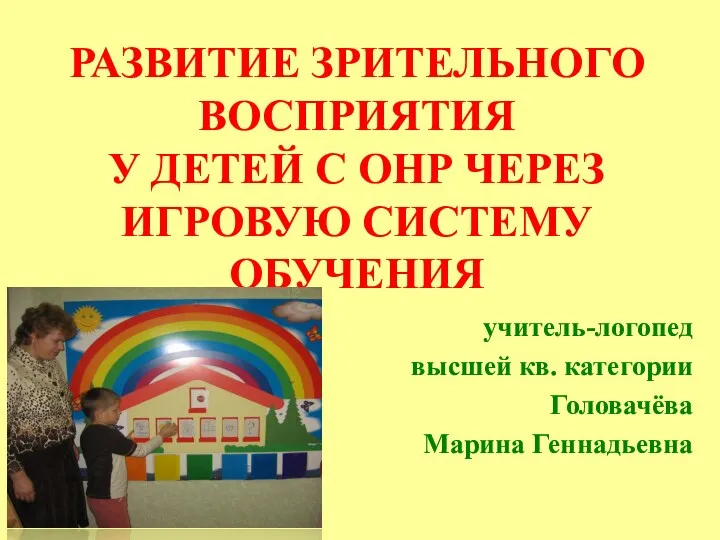 Развитие зрительного восприятия у детей с ОНР через игровую систему обучения
 Кітап оқуға баулу
 Летний профильный отряд по химии Волшебный мир химии
 Древняя Индия
 Ұлпа қабынуын емдеудің салыстырмалы сипаттамасы
 Требования к хорошему кейсу
 Как семейные традиции укрепляют семью
 Послеродовые гнойно-септические заболевания (перитонит, сепсис, токсико-инфекционный шок)
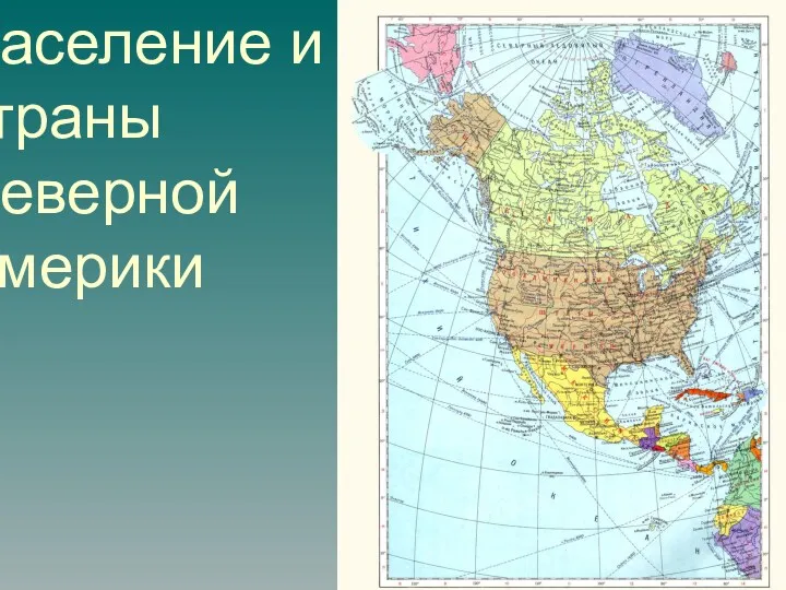 7 класс: Население и страны Северной Америки