- M&M: The Starting Point

Содержание
- 2. FIN 591: Financial Fundamentals/Valuation M&M: The Starting Point A number of restrictive assumptions apply Use the
- 3. FIN 591: Financial Fundamentals/Valuation The M&M Assumptions Homogeneous expectations Homogeneous business risk (σEBIT) classes Perpetual no-growth
- 4. FIN 591: Financial Fundamentals/Valuation Business Risk Business risk: Risk surrounding expected operating cash flows Factors causing
- 5. FIN 591: Financial Fundamentals/Valuation Principle of Additivity Allows you to value the cash flows in any
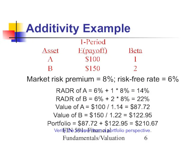
- 6. FIN 591: Financial Fundamentals/Valuation Additivity Example Market risk premium = 8%; risk-free rate = 6% RADR
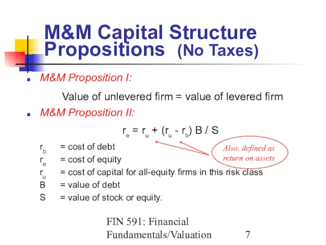
- 7. FIN 591: Financial Fundamentals/Valuation M&M Capital Structure Propositions (No Taxes) M&M Proposition I: Value of unlevered
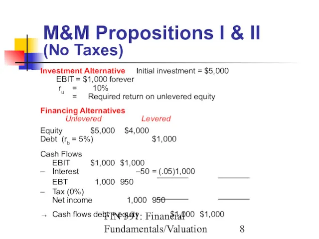
- 8. FIN 591: Financial Fundamentals/Valuation M&M Propositions I & II (No Taxes) Investment Alternative Initial investment =
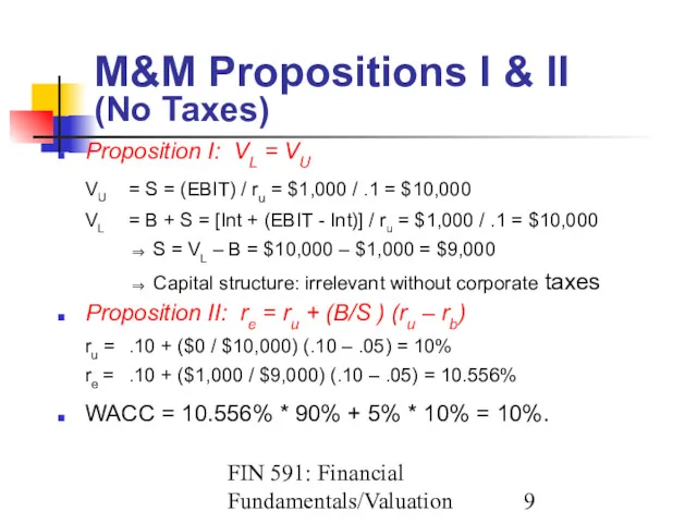
- 9. FIN 591: Financial Fundamentals/Valuation M&M Propositions I & II (No Taxes) Proposition I: VL = VU
- 10. FIN 591: Financial Fundamentals/Valuation Graphing the M&M No-Tax Relationships Firm value (Proposition I) VU VL Debt
- 11. FIN 591: Financial Fundamentals/Valuation M&M Capital Structure Propositions (Corporate Taxes) M&M Proposition I: VL = VU
- 12. FIN 591: Financial Fundamentals/Valuation M&M Propositions I & II (Corporate Taxes) Investment and financing alternatives -
- 13. FIN 591: Financial Fundamentals/Valuation Tax Benefit of Debt Financing Debt interest is tax deductible For every
- 14. FIN 591: Financial Fundamentals/Valuation A Look at the Propositions Proposition I: VL = VU + τC
- 15. FIN 591: Financial Fundamentals/Valuation Confirmation VL = B + S = rb B / rb +
- 16. FIN 591: Financial Fundamentals/Valuation Graphing the M&M Relationships Firm value (Proposition I) VL Slope = τc
- 17. FIN 591: Financial Fundamentals/Valuation Another Look with Corporate Taxes Market Value Balance Sheet (All equity firm)
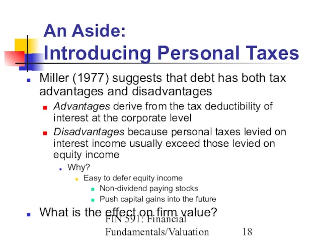
- 18. FIN 591: Financial Fundamentals/Valuation An Aside: Introducing Personal Taxes Miller (1977) suggests that debt has both
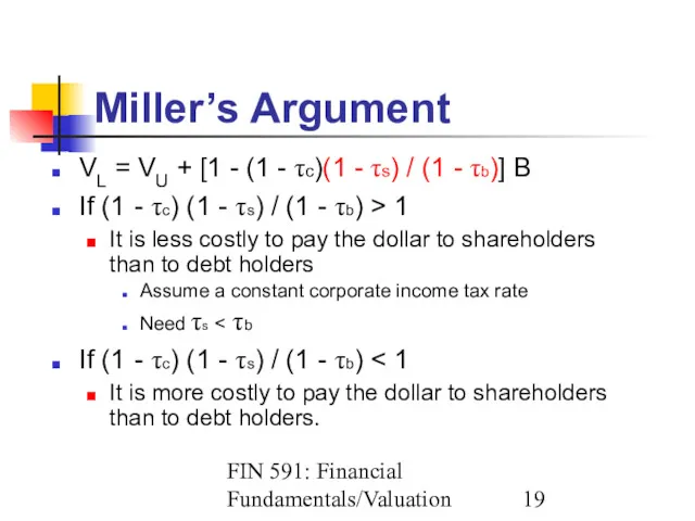
- 19. FIN 591: Financial Fundamentals/Valuation Miller’s Argument VL = VU + [1 - (1 - τc)(1 -
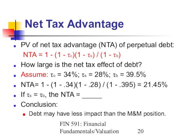
- 20. FIN 591: Financial Fundamentals/Valuation Net Tax Advantage PV of net tax advantage (NTA) of perpetual debt:
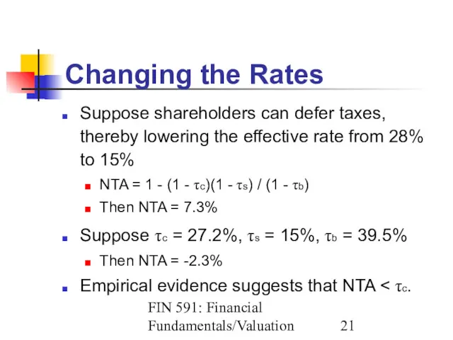
- 21. FIN 591: Financial Fundamentals/Valuation Changing the Rates Suppose shareholders can defer taxes, thereby lowering the effective
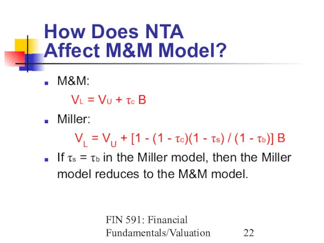
- 22. FIN 591: Financial Fundamentals/Valuation How Does NTA Affect M&M Model? M&M: VL = VU + τc
- 23. FIN 591: Financial Fundamentals/Valuation A Graphical View of Miller Value Vu Debt (B) VL = VU
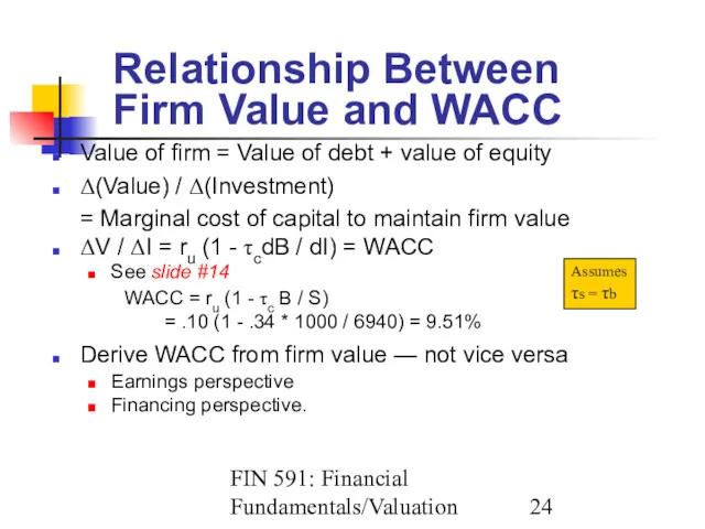
- 24. FIN 591: Financial Fundamentals/Valuation Relationship Between Firm Value and WACC Value of firm = Value of
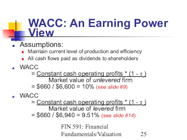
- 25. FIN 591: Financial Fundamentals/Valuation WACC: An Earning Power View Assumptions: Maintain current level of production and
- 26. FIN 591: Financial Fundamentals/Valuation WACC: A Financing View Calculate the cost of: Debt Preferred stock Common
- 27. FIN 591: Financial Fundamentals/Valuation Debt’s Yield to Maturity Example: 14s of December 2014 selling for 110
- 28. FIN 591: Financial Fundamentals/Valuation A Graphical View: YTM Semiannual interest rate (r) $2,610 $2,000 $1,100 $1,000
- 29. FIN 591: Financial Fundamentals/Valuation Cost of Debt Cost of debt to the firm is the YTM
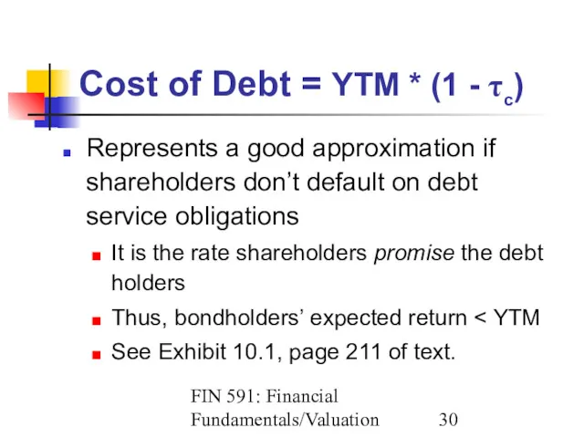
- 30. FIN 591: Financial Fundamentals/Valuation Cost of Debt = YTM * (1 - τc) Represents a good
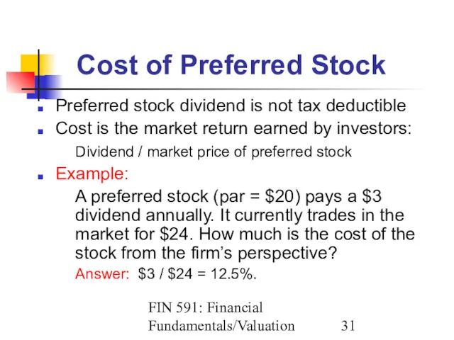
- 31. FIN 591: Financial Fundamentals/Valuation Cost of Preferred Stock Preferred stock dividend is not tax deductible Cost
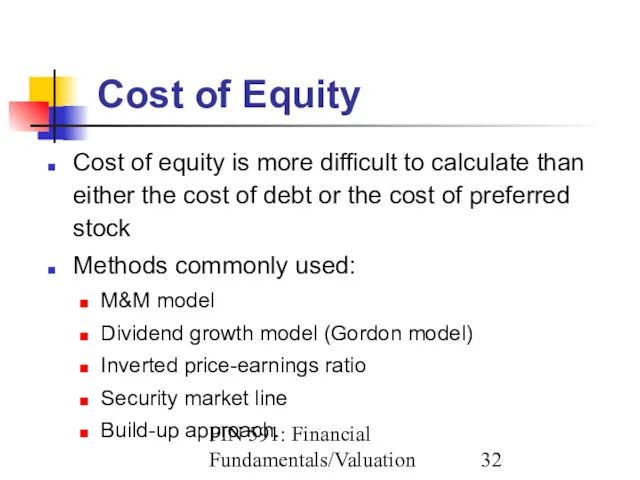
- 32. FIN 591: Financial Fundamentals/Valuation Cost of Equity Cost of equity is more difficult to calculate than
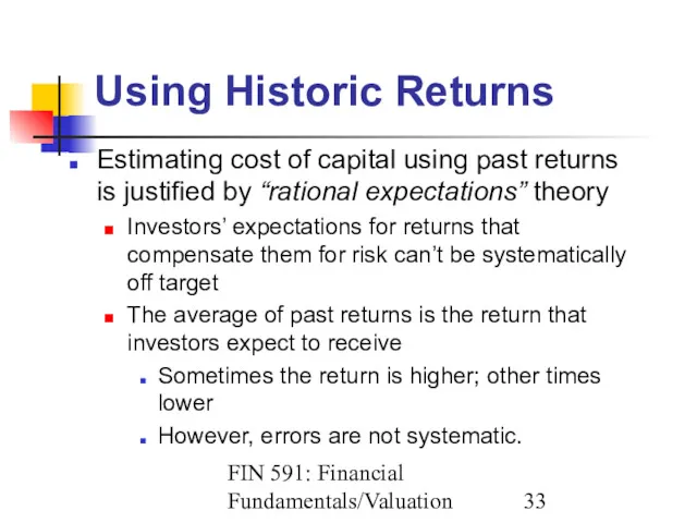
- 33. FIN 591: Financial Fundamentals/Valuation Using Historic Returns Estimating cost of capital using past returns is justified
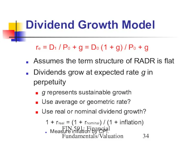
- 34. FIN 591: Financial Fundamentals/Valuation Dividend Growth Model re = D1 / P0 + g = D0
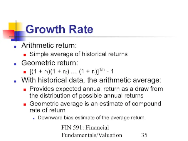
- 35. FIN 591: Financial Fundamentals/Valuation Growth Rate Arithmetic return: Simple average of historical returns Geometric return: [(1
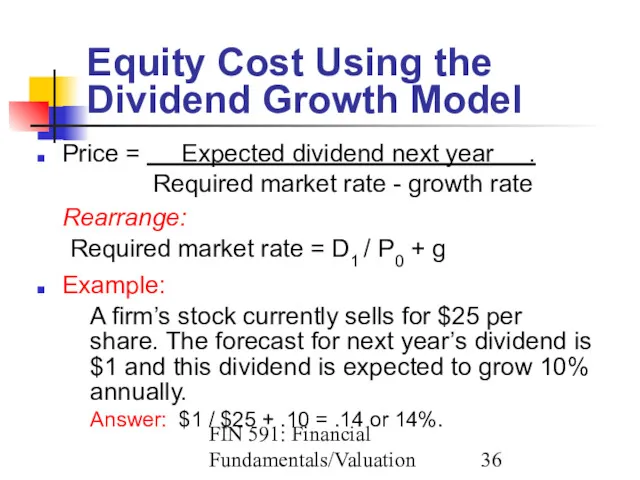
- 36. FIN 591: Financial Fundamentals/Valuation Equity Cost Using the Dividend Growth Model Price = Expected dividend next
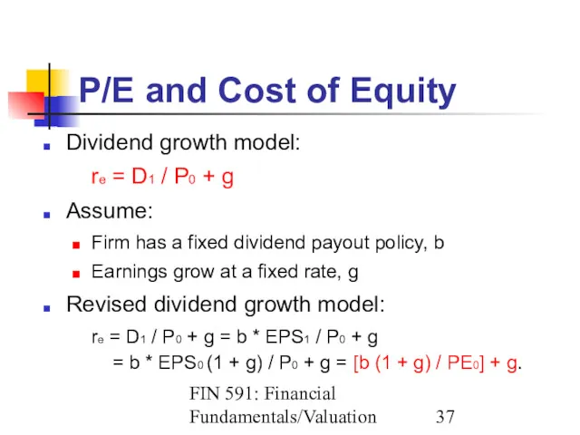
- 37. FIN 591: Financial Fundamentals/Valuation P/E and Cost of Equity Dividend growth model: re = D1 /
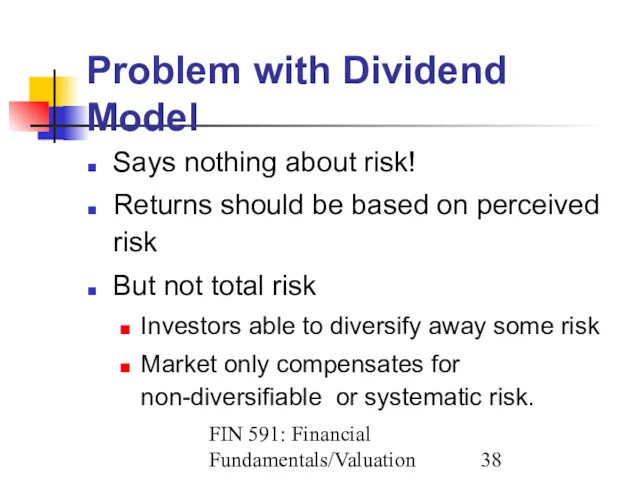
- 38. FIN 591: Financial Fundamentals/Valuation Problem with Dividend Model Says nothing about risk! Returns should be based
- 40. Скачать презентацию
FIN 591: Financial Fundamentals/Valuation
M&M: The Starting Point
A number of restrictive assumptions
FIN 591: Financial Fundamentals/Valuation
M&M: The Starting Point
A number of restrictive assumptions
FIN 591: Financial Fundamentals/Valuation
The M&M Assumptions
Homogeneous expectations
Homogeneous business risk (σEBIT) classes
Perpetual
FIN 591: Financial Fundamentals/Valuation
The M&M Assumptions
Homogeneous expectations
Homogeneous business risk (σEBIT) classes
Perpetual
FIN 591: Financial Fundamentals/Valuation
Business Risk
Business risk:
Risk surrounding expected operating cash flows
Factors
FIN 591: Financial Fundamentals/Valuation
Business Risk
Business risk:
Risk surrounding expected operating cash flows
Factors
FIN 591: Financial Fundamentals/Valuation
Principle of Additivity
Allows you to value the cash
FIN 591: Financial Fundamentals/Valuation
Principle of Additivity
Allows you to value the cash
FIN 591: Financial Fundamentals/Valuation
Additivity Example
Market risk premium = 8%; risk-free rate
FIN 591: Financial Fundamentals/Valuation
Additivity Example
Market risk premium = 8%; risk-free rate
FIN 591: Financial Fundamentals/Valuation
M&M Capital Structure Propositions (No Taxes)
M&M Proposition
FIN 591: Financial Fundamentals/Valuation
M&M Capital Structure Propositions (No Taxes)
M&M Proposition
FIN 591: Financial Fundamentals/Valuation
M&M Propositions I & II
(No Taxes)
Investment Alternative
FIN 591: Financial Fundamentals/Valuation
M&M Propositions I & II
(No Taxes)
Investment Alternative
FIN 591: Financial Fundamentals/Valuation
M&M Propositions I & II
(No Taxes)
Proposition I:
FIN 591: Financial Fundamentals/Valuation
M&M Propositions I & II
(No Taxes)
Proposition I:
FIN 591: Financial Fundamentals/Valuation
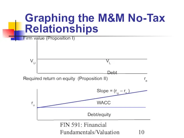
Graphing the M&M No-Tax Relationships
Firm value (Proposition
FIN 591: Financial Fundamentals/Valuation
Graphing the M&M No-Tax Relationships
Firm value (Proposition
FIN 591: Financial Fundamentals/Valuation
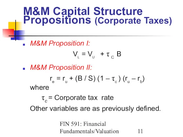
M&M Capital Structure Propositions (Corporate Taxes)
M&M Proposition I:
VL
FIN 591: Financial Fundamentals/Valuation
M&M Capital Structure Propositions (Corporate Taxes)
M&M Proposition I:
VL
FIN 591: Financial Fundamentals/Valuation
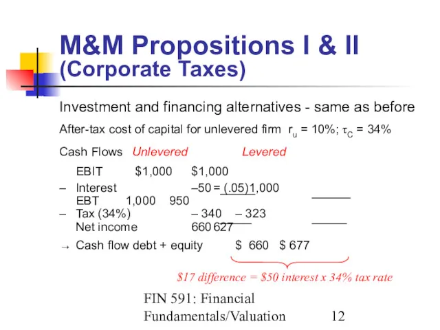
M&M Propositions I & II (Corporate Taxes)
Investment and
FIN 591: Financial Fundamentals/Valuation
M&M Propositions I & II (Corporate Taxes)
Investment and
FIN 591: Financial Fundamentals/Valuation
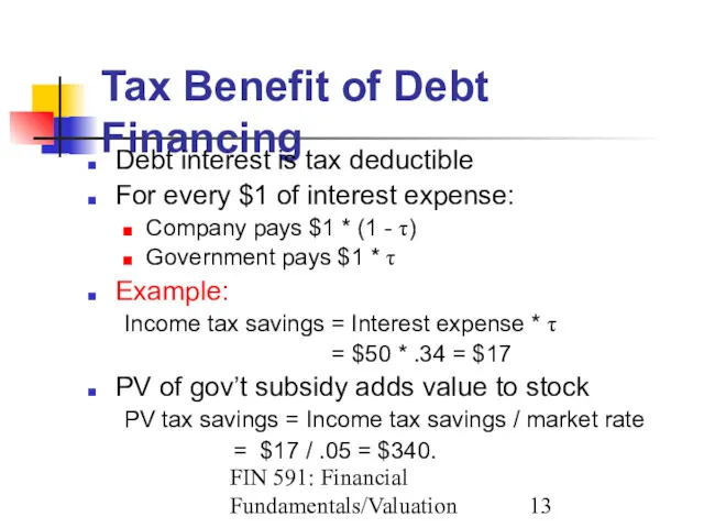
Tax Benefit of Debt Financing
Debt interest is tax
FIN 591: Financial Fundamentals/Valuation
Tax Benefit of Debt Financing
Debt interest is tax
FIN 591: Financial Fundamentals/Valuation
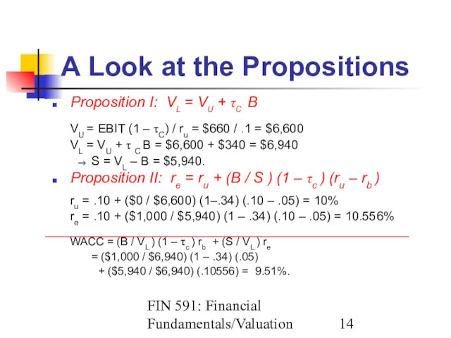
A Look at the Propositions
Proposition I: VL =
FIN 591: Financial Fundamentals/Valuation
A Look at the Propositions
Proposition I: VL =
FIN 591: Financial Fundamentals/Valuation
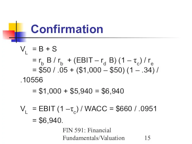
Confirmation
VL = B + S
= rb B / rb
FIN 591: Financial Fundamentals/Valuation
Confirmation
VL = B + S
= rb B / rb
FIN 591: Financial Fundamentals/Valuation
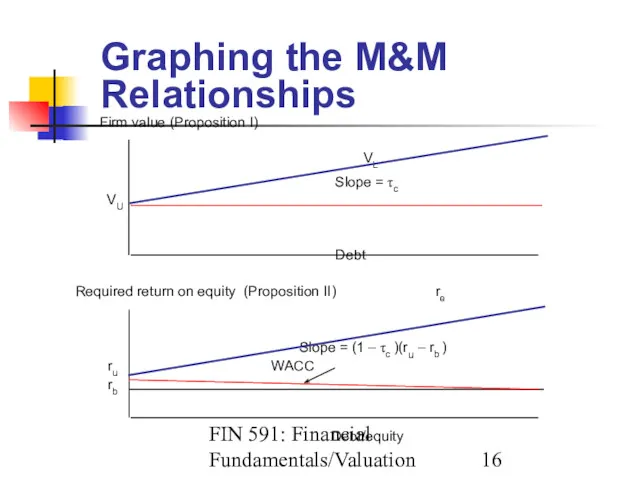
Graphing the M&M Relationships
Firm value (Proposition I)
FIN 591: Financial Fundamentals/Valuation
Graphing the M&M Relationships
Firm value (Proposition I)
FIN 591: Financial Fundamentals/Valuation
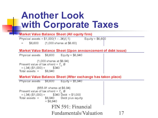
Another Look
with Corporate Taxes
Market Value Balance Sheet (All
FIN 591: Financial Fundamentals/Valuation
Another Look
with Corporate Taxes
Market Value Balance Sheet (All
FIN 591: Financial Fundamentals/Valuation
An Aside:
Introducing Personal Taxes
Miller (1977) suggests that debt
FIN 591: Financial Fundamentals/Valuation
An Aside:
Introducing Personal Taxes
Miller (1977) suggests that debt
FIN 591: Financial Fundamentals/Valuation
Miller’s Argument
VL = VU + [1 - (1
FIN 591: Financial Fundamentals/Valuation
Miller’s Argument
VL = VU + [1 - (1
FIN 591: Financial Fundamentals/Valuation
Net Tax Advantage
PV of net tax advantage (NTA)
FIN 591: Financial Fundamentals/Valuation
Net Tax Advantage
PV of net tax advantage (NTA)
FIN 591: Financial Fundamentals/Valuation
Changing the Rates
Suppose shareholders can defer taxes, thereby
FIN 591: Financial Fundamentals/Valuation
Changing the Rates
Suppose shareholders can defer taxes, thereby
FIN 591: Financial Fundamentals/Valuation
How Does NTA
Affect M&M Model?
M&M:
VL = VU +
FIN 591: Financial Fundamentals/Valuation
How Does NTA
Affect M&M Model?
M&M:
VL = VU +
FIN 591: Financial Fundamentals/Valuation
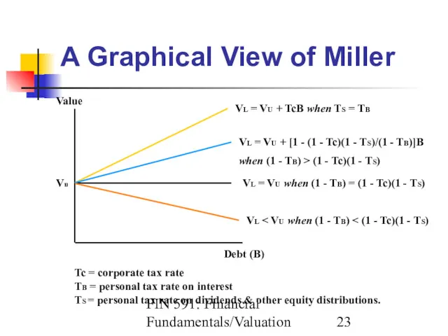
A Graphical View of Miller
Value
Vu
Debt (B)
VL = VU
FIN 591: Financial Fundamentals/Valuation
A Graphical View of Miller
Value
Vu
Debt (B)
VL = VU
FIN 591: Financial Fundamentals/Valuation
Relationship Between
Firm Value and WACC
Value of firm
FIN 591: Financial Fundamentals/Valuation
Relationship Between
Firm Value and WACC
Value of firm
FIN 591: Financial Fundamentals/Valuation
WACC: An Earning Power View
Assumptions:
Maintain current level of
FIN 591: Financial Fundamentals/Valuation
WACC: An Earning Power View
Assumptions:
Maintain current level of
FIN 591: Financial Fundamentals/Valuation
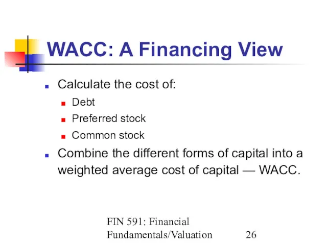
WACC: A Financing View
Calculate the cost of:
Debt
Preferred stock
Common
FIN 591: Financial Fundamentals/Valuation
WACC: A Financing View
Calculate the cost of:
Debt
Preferred stock
Common
FIN 591: Financial Fundamentals/Valuation
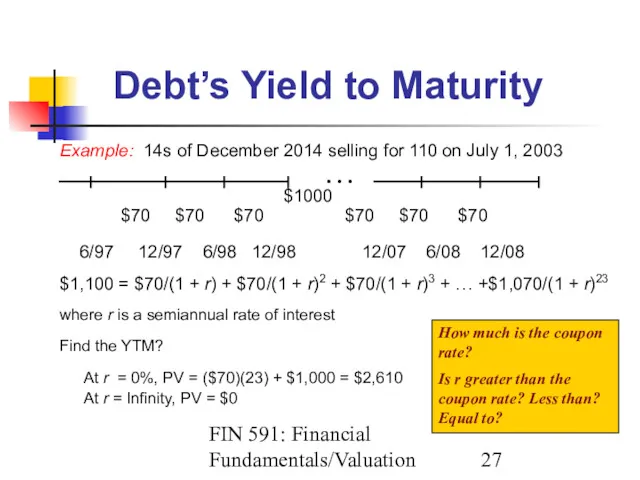
Debt’s Yield to Maturity
Example: 14s of December 2014
FIN 591: Financial Fundamentals/Valuation
Debt’s Yield to Maturity
Example: 14s of December 2014
FIN 591: Financial Fundamentals/Valuation
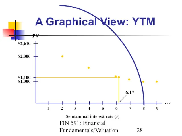
A Graphical View: YTM
Semiannual interest rate (r)
$2,610
$2,000
$1,100
$1,000
1 2
FIN 591: Financial Fundamentals/Valuation
A Graphical View: YTM
Semiannual interest rate (r)
$2,610
$2,000
$1,100
$1,000
1 2
FIN 591: Financial Fundamentals/Valuation
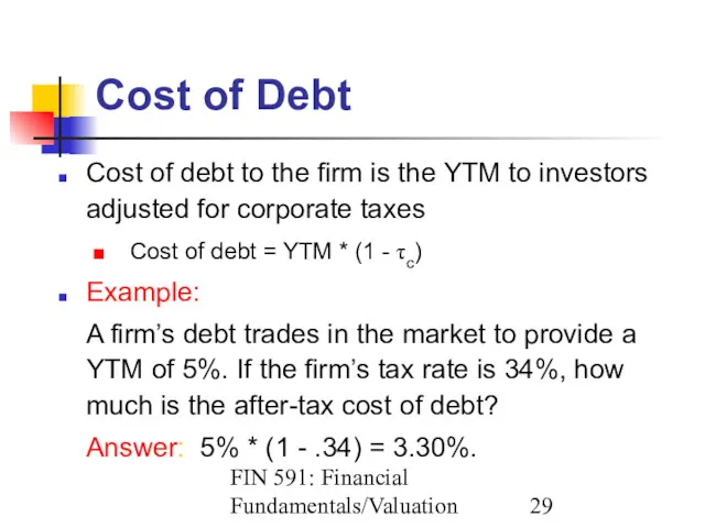
Cost of Debt
Cost of debt to the firm
FIN 591: Financial Fundamentals/Valuation
Cost of Debt
Cost of debt to the firm
FIN 591: Financial Fundamentals/Valuation
Cost of Debt = YTM * (1 -
FIN 591: Financial Fundamentals/Valuation
Cost of Debt = YTM * (1 -
FIN 591: Financial Fundamentals/Valuation
Cost of Preferred Stock
Preferred stock dividend is not
FIN 591: Financial Fundamentals/Valuation
Cost of Preferred Stock
Preferred stock dividend is not
FIN 591: Financial Fundamentals/Valuation
Cost of Equity
Cost of equity is more difficult
FIN 591: Financial Fundamentals/Valuation
Cost of Equity
Cost of equity is more difficult
FIN 591: Financial Fundamentals/Valuation
Using Historic Returns
Estimating cost of capital using past
FIN 591: Financial Fundamentals/Valuation
Using Historic Returns
Estimating cost of capital using past
FIN 591: Financial Fundamentals/Valuation
Dividend Growth Model
re = D1 / P0 +
FIN 591: Financial Fundamentals/Valuation
Dividend Growth Model
re = D1 / P0 +
FIN 591: Financial Fundamentals/Valuation
Growth Rate
Arithmetic return:
Simple average of historical returns
Geometric return:
[(1
FIN 591: Financial Fundamentals/Valuation
Growth Rate
Arithmetic return:
Simple average of historical returns
Geometric return:
[(1
FIN 591: Financial Fundamentals/Valuation
Equity Cost Using the
Dividend Growth Model
Price =
FIN 591: Financial Fundamentals/Valuation
Equity Cost Using the
Dividend Growth Model
Price =
FIN 591: Financial Fundamentals/Valuation
P/E and Cost of Equity
Dividend growth model:
re =
FIN 591: Financial Fundamentals/Valuation
P/E and Cost of Equity
Dividend growth model:
re =
FIN 591: Financial Fundamentals/Valuation
Problem with Dividend Model
Says nothing about risk!
Returns should
FIN 591: Financial Fundamentals/Valuation
Problem with Dividend Model
Says nothing about risk!
Returns should
 Новые правила грамматики английского языка
 London attractions
 Infinitive. The negative infinitive. The present infinitive
 Интерактивные методы обучения как способ формирования коммуникативной компетенции учащихся при изучении английского языка
 The Beatles music
 Future Tenses
 Косвенная речь
 All about volcanoes
 Present Continuous mine
 Неопределенный артикль, 5 класс
 Language and culture
 We are having a great time!
 Body parts
 Everyday products
 Wh-questions vk interactive english
 Using games in a foreign language classroom
 The impact of discrimination on culture
 The Verb
 Present Simple
 Leisure and entertainment
 Big Ben
 Hello, kids! Hello September
 Игра-викторина по английскому языку
 Rotordynamics
 Leisure Activities. Vocabulary
 Причастие – неличная форма глагола, сочетающая свойства глагола, прилагательного и наречия
 Трудности перевода терминов
 Distinctive features of the functional styles. Lecture 10