- Synchronous Machines Models

Содержание
- 2. Announcements Homework 2 is due now Homework 3 is on the website and is due on
- 3. Single Machine, Infinite Bus System (SMIB) Book introduces new variables by combining machine values with line
- 4. “Transient Speed” Mechanical time constant A small parameter Introduce New Constants We are ignoring the exciter
- 5. Stator Flux Differential Equations
- 6. An exact integral manifold (for any sized ε): Special Case of Zero Resistance Without resistance this
- 7. Direct Axis Equations
- 8. Quadrature Axis Equations
- 9. Swing Equations These are equivalent to the more traditional swing expressions
- 10. Stator Flux Expressions
- 11. Network Expressions
- 12. 3 fast dynamic states 6 not so fast dynamic states 8 algebraic states Machine Variable Summary
- 13. Elimination of Stator Transients If we assume the stator flux equations are much faster than the
- 14. Impact on Studies Image Source: P. Kundur, Power System Stability and Control, EPRI, McGraw-Hill, 1994
- 15. Stator Flux Expressions
- 16. Network Constraints
- 17. "Interesting" Dynamic Circuit
- 18. These last two equations can be written as one complex equation. "Interesting" Dynamic Circuit
- 19. Subtransient Algebraic Circuit
- 20. Subtransient Algebraic Circuit Subtransient saliency use to be ignored (i.e., assuming X"q=X"d). However that is increasingly
- 21. Simplified Machine Models Often more simplified models were used to represent synchronous machines These simplifications are
- 22. Two-Axis Model If we assume the damper winding dynamics are sufficiently fast, then T"do and T"qo
- 23. Two-Axis Model Then
- 24. Two-Axis Model And
- 25. Two-Axis Model
- 26. Two-Axis Model No saturation effects are included with this model
- 27. Two-Axis Model
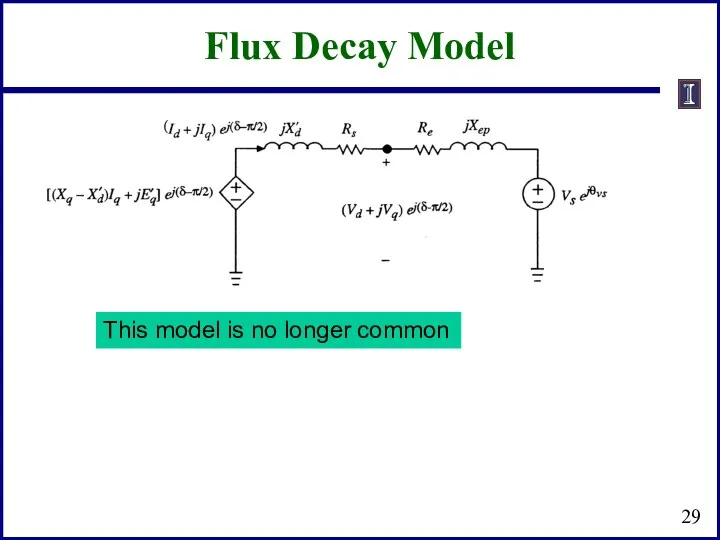
- 28. Flux Decay Model If we assume T'qo is sufficiently fast then
- 29. Flux Decay Model This model is no longer common
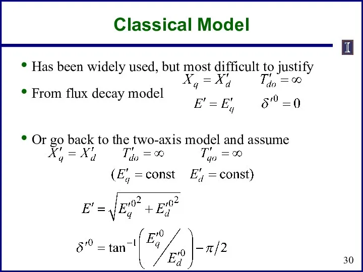
- 30. Classical Model Has been widely used, but most difficult to justify From flux decay model Or
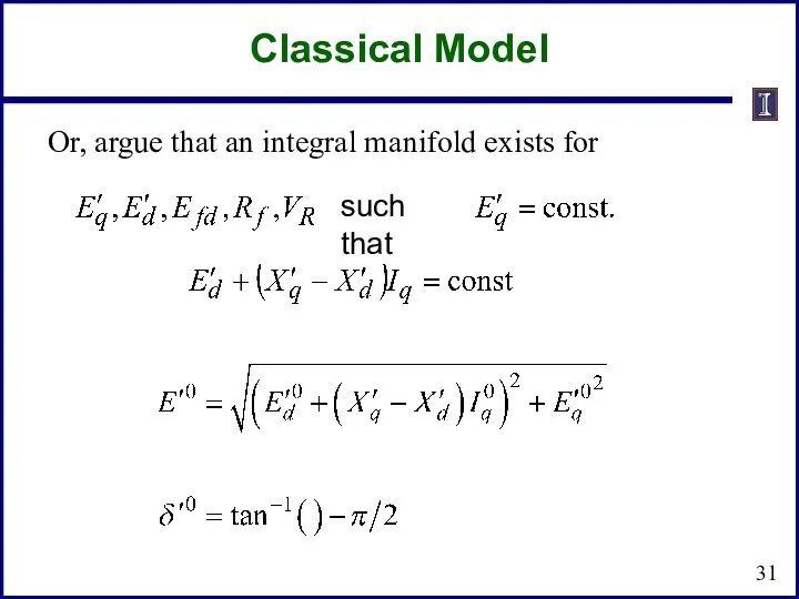
- 31. Or, argue that an integral manifold exists for such that Classical Model
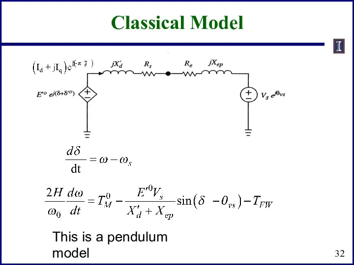
- 32. Classical Model This is a pendulum model
- 33. Full model with stator transients Sub-transient model Two-axis model One-axis model Classical model (const. E behind
- 34. Damping Torques Friction and windage Usually small Stator currents (load) Usually represented in the load models
- 35. Industrial Models There are just a handful of synchronous machine models used in North America GENSAL
- 36. Network Reference Frame In transient stability the initial generator values are set from a power flow
- 37. Network Reference Frame Issue of calculating δ, which is key, will be considered for each model
- 38. Two-Axis Model We'll start with the PowerWorld two-axis model (two-axis models are not common commercially, but
- 39. Two-Axis Model Value of δ is determined from (3.229 from book) Once δ is determined then
- 40. Example (Used for All Models) Below example will be used with all models. Assume a 100
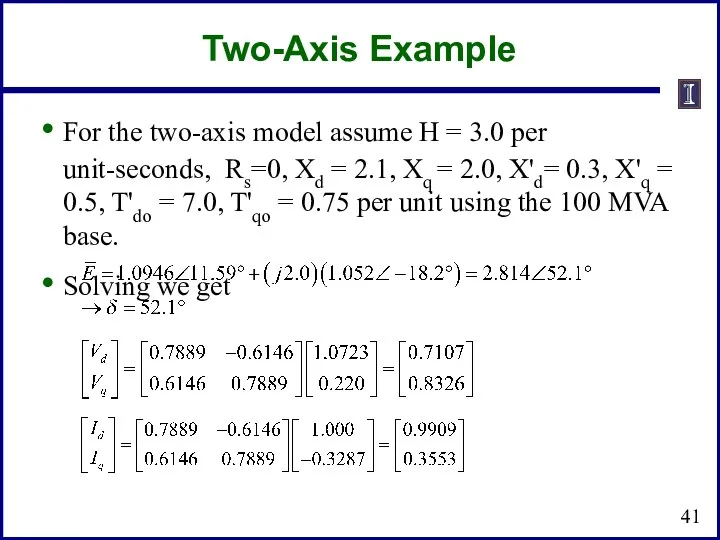
- 41. Two-Axis Example For the two-axis model assume H = 3.0 per unit-seconds, Rs=0, Xd = 2.1,
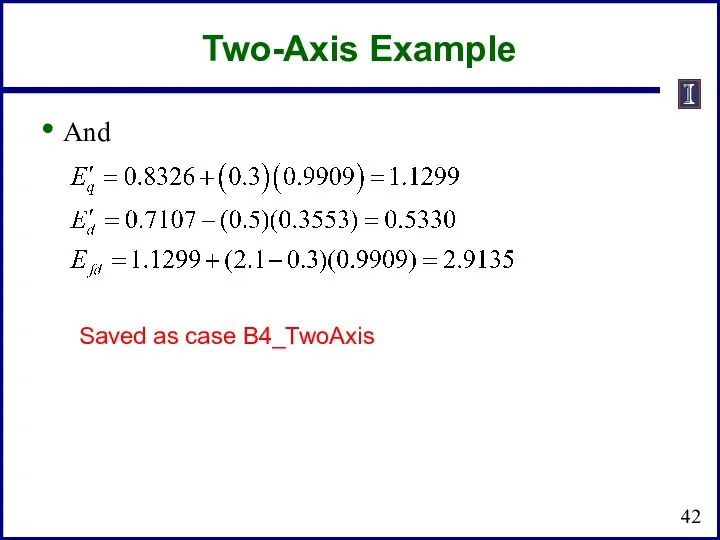
- 42. Two-Axis Example And Saved as case B4_TwoAxis
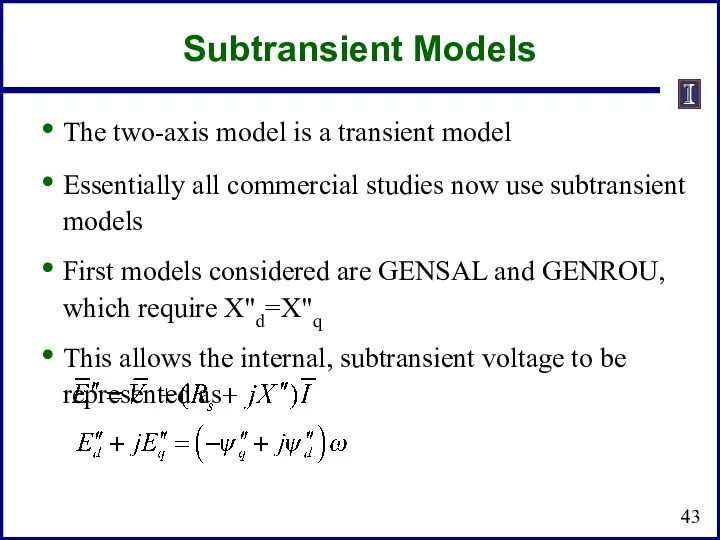
- 43. Subtransient Models The two-axis model is a transient model Essentially all commercial studies now use subtransient
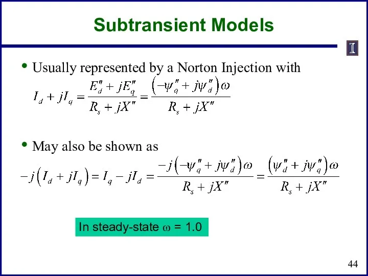
- 44. Subtransient Models Usually represented by a Norton Injection with May also be shown as In steady-state
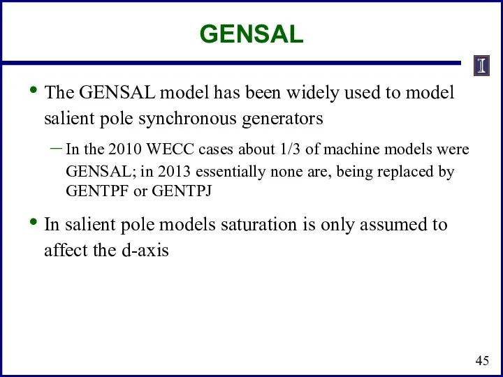
- 45. GENSAL The GENSAL model has been widely used to model salient pole synchronous generators In the
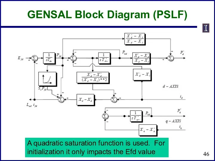
- 46. GENSAL Block Diagram (PSLF) A quadratic saturation function is used. For initialization it only impacts the
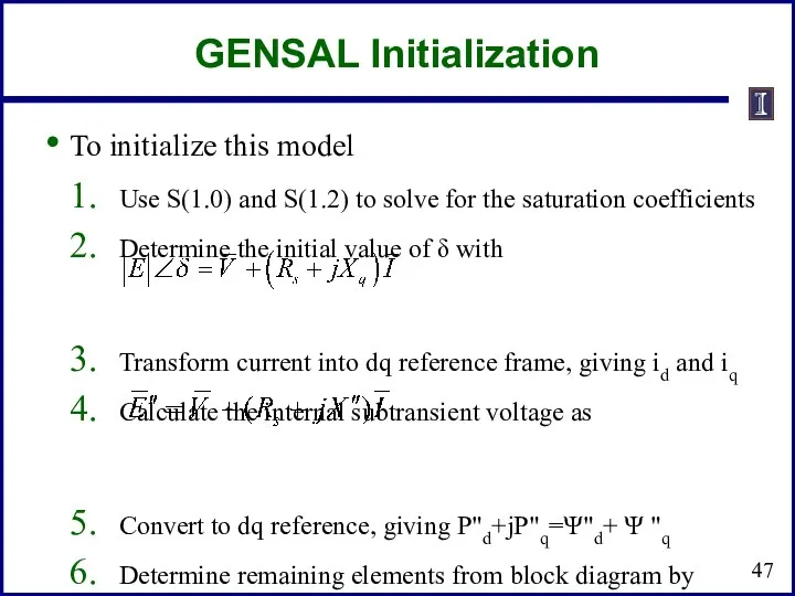
- 47. GENSAL Initialization To initialize this model Use S(1.0) and S(1.2) to solve for the saturation coefficients
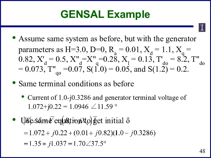
- 48. GENSAL Example Assume same system as before, but with the generator parameters as H=3.0, D=0, Ra
- 49. GENSAL Example Then And
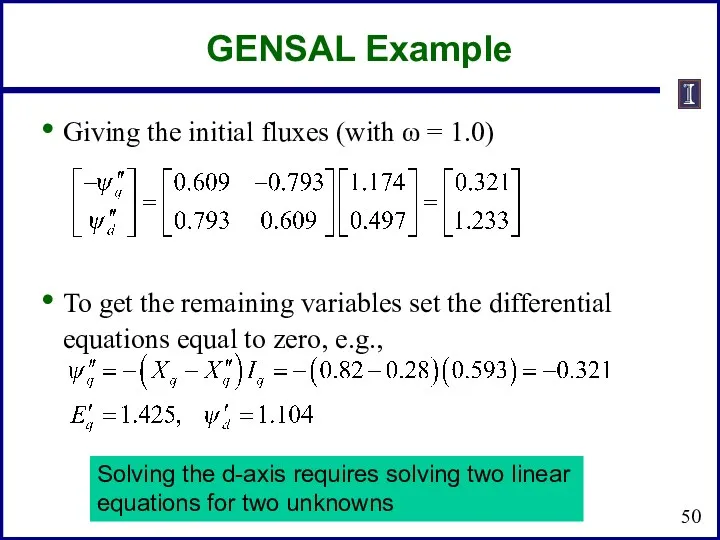
- 50. GENSAL Example Giving the initial fluxes (with ω = 1.0) To get the remaining variables set
- 52. Скачать презентацию

Announcements
Homework 2 is due now
Homework 3 is on the website and
Announcements
Homework 2 is due now
Homework 3 is on the website and
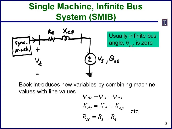
Single Machine, Infinite Bus System (SMIB)
Book introduces new variables by combining
Single Machine, Infinite Bus System (SMIB)
Book introduces new variables by combining
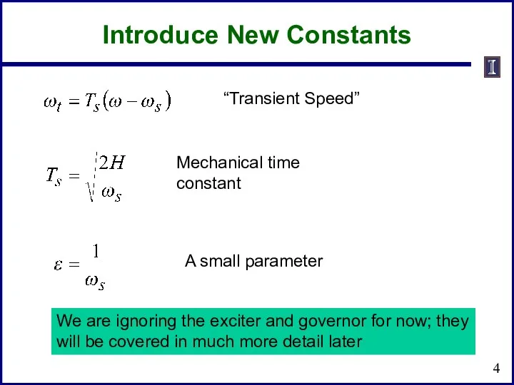
“Transient Speed”
Mechanical time constant
A small parameter
Introduce New Constants
We are ignoring the
“Transient Speed”
Mechanical time constant
A small parameter
Introduce New Constants
We are ignoring the
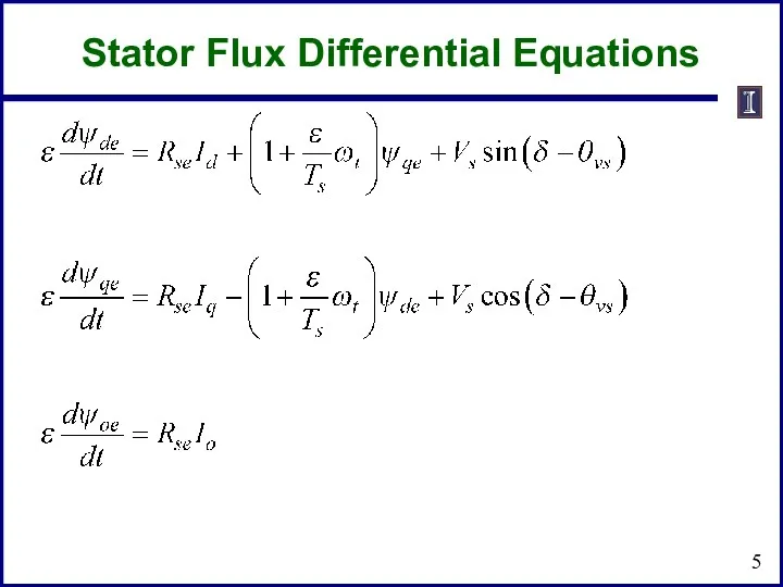
Stator Flux Differential Equations
Stator Flux Differential Equations
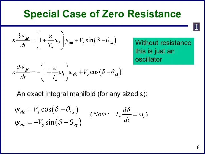
An exact integral manifold (for any sized ε):
Special Case of Zero
An exact integral manifold (for any sized ε):
Special Case of Zero
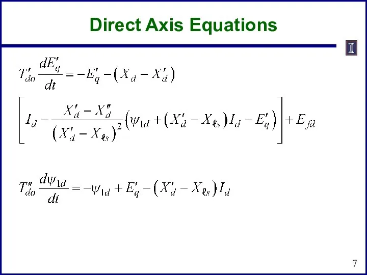
Direct Axis Equations
Direct Axis Equations
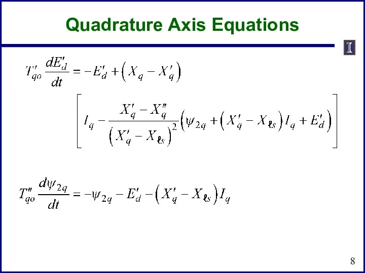
Quadrature Axis Equations
Quadrature Axis Equations
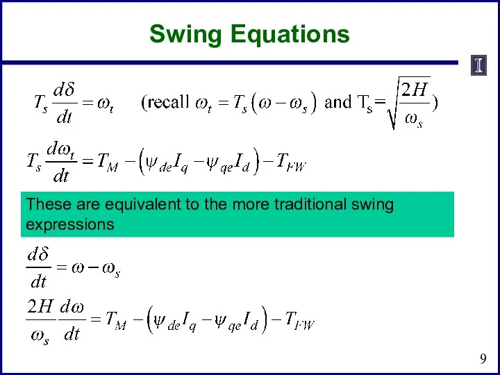
Swing Equations
These are equivalent to the more traditional swing expressions
Swing Equations
These are equivalent to the more traditional swing expressions
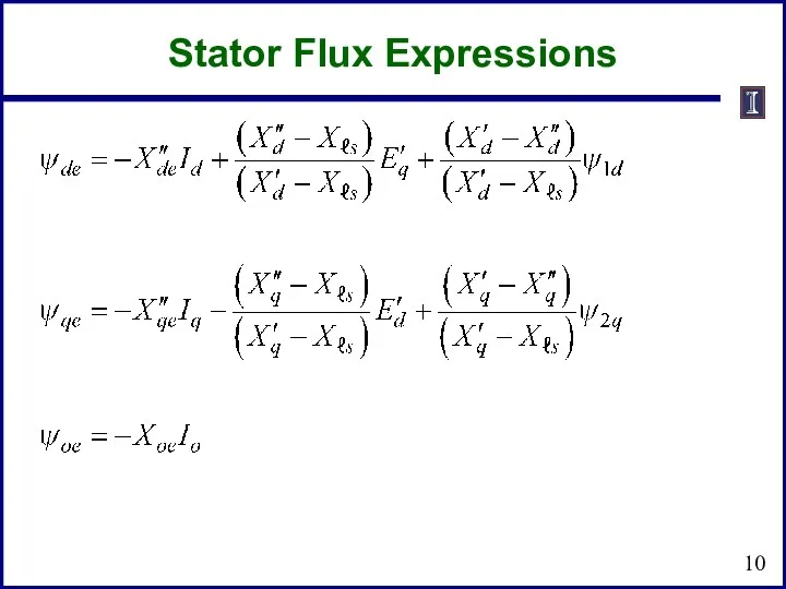
Stator Flux Expressions
Stator Flux Expressions
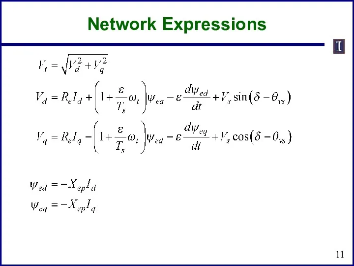
Network Expressions
Network Expressions
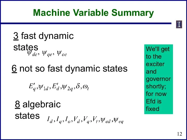
3 fast dynamic states
6 not so fast dynamic states
8 algebraic states
Machine
3 fast dynamic states
6 not so fast dynamic states
8 algebraic states
Machine
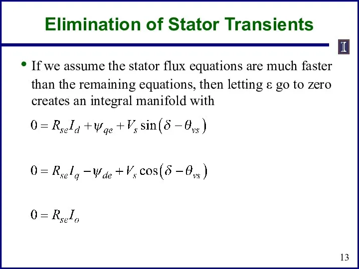
Elimination of Stator Transients
If we assume the stator flux equations are
Elimination of Stator Transients
If we assume the stator flux equations are
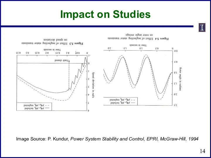
Impact on Studies
Image Source: P. Kundur, Power System Stability and Control,
Impact on Studies
Image Source: P. Kundur, Power System Stability and Control,

Stator Flux Expressions
Stator Flux Expressions
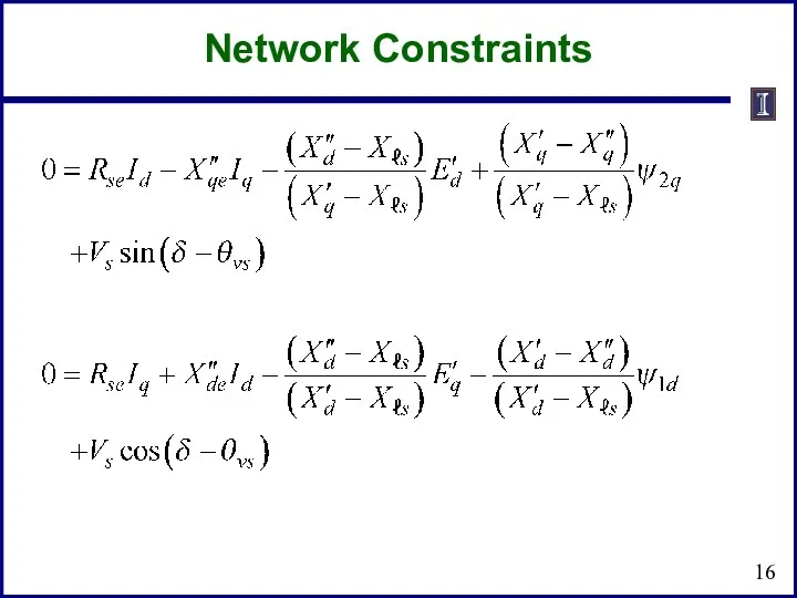
Network Constraints
Network Constraints
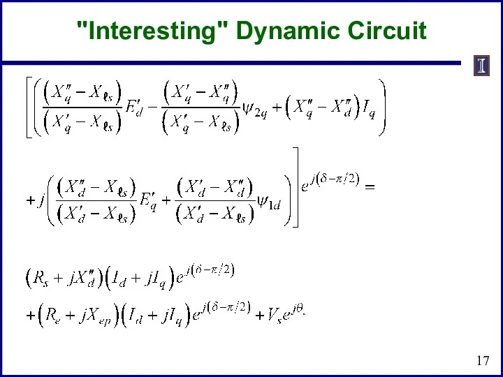
"Interesting" Dynamic Circuit
"Interesting" Dynamic Circuit
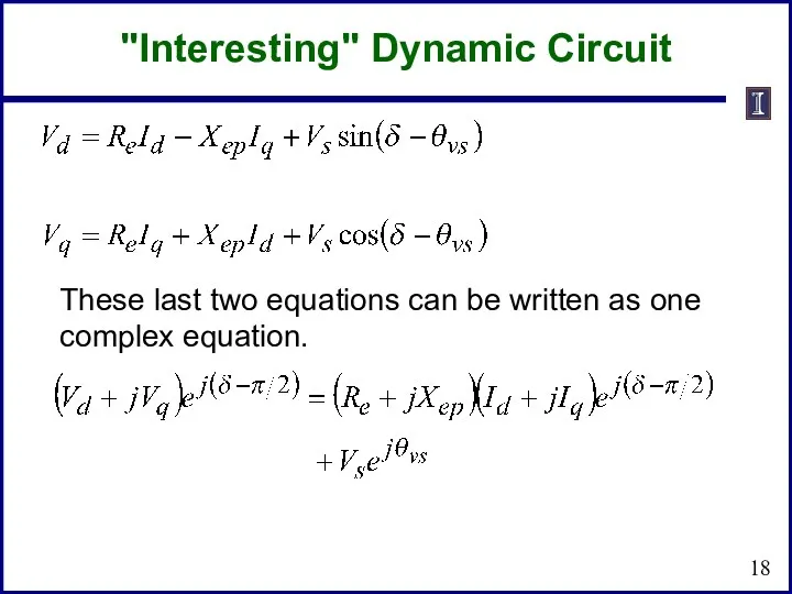
These last two equations can be written as one complex equation.
"Interesting"
These last two equations can be written as one complex equation.
"Interesting"
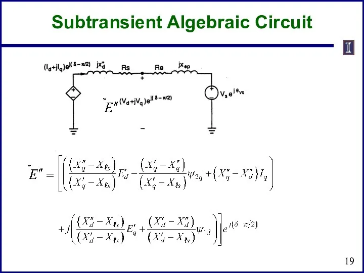
Subtransient Algebraic Circuit
Subtransient Algebraic Circuit
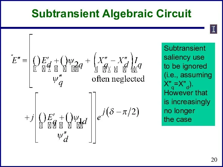
Subtransient Algebraic Circuit
Subtransient
saliency use
to be ignored
(i.e., assuming
X"q=X"d).
However that
is increasingly
no longer
the
Subtransient Algebraic Circuit
Subtransient saliency use to be ignored (i.e., assuming X"q=X"d). However that is increasingly no longer the
Simplified Machine Models
Often more simplified models were used to represent synchronous
Simplified Machine Models
Often more simplified models were used to represent synchronous

Two-Axis Model
If we assume the damper winding dynamics are sufficiently fast,
Two-Axis Model
If we assume the damper winding dynamics are sufficiently fast,
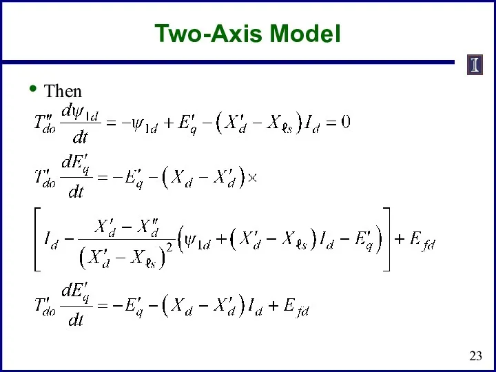
Two-Axis Model
Then
Two-Axis Model
Then
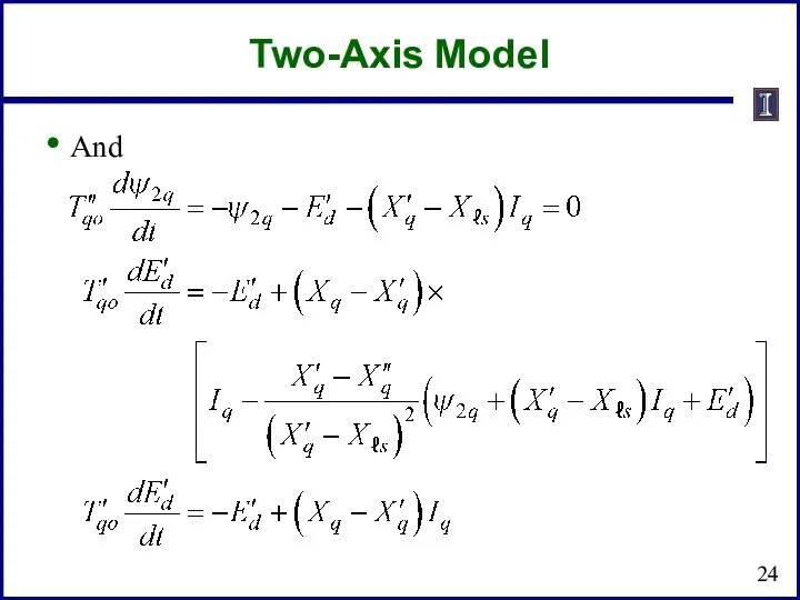
Two-Axis Model
And
Two-Axis Model
And
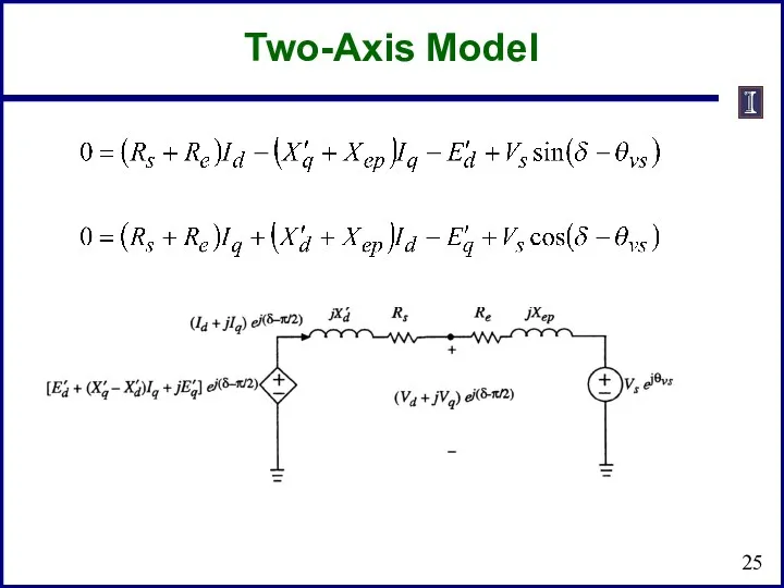
Two-Axis Model
Two-Axis Model
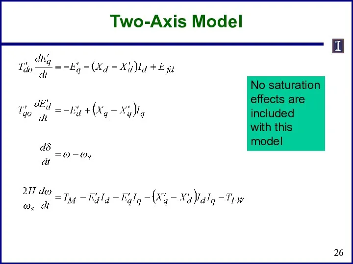
Two-Axis Model
No saturation
effects are
included
with this
model
Two-Axis Model
No saturation
effects are
included
with this
model
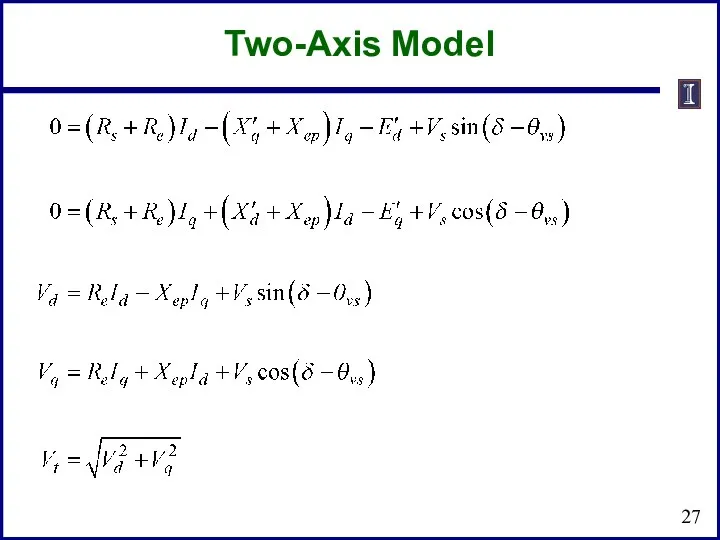
Two-Axis Model
Two-Axis Model
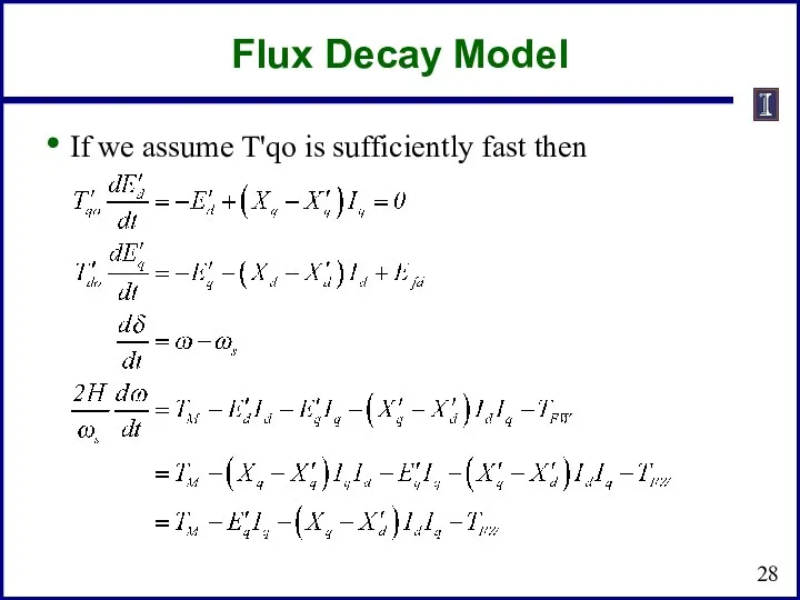
Flux Decay Model
If we assume T'qo is sufficiently fast then
Flux Decay Model
If we assume T'qo is sufficiently fast then
Flux Decay Model
This model is no longer common
Flux Decay Model
This model is no longer common
Classical Model
Has been widely used, but most difficult to justify
From flux
Classical Model
Has been widely used, but most difficult to justify
From flux
Or, argue that an integral manifold exists for
such that
Classical Model
Or, argue that an integral manifold exists for
such that
Classical Model
Classical Model
This is a pendulum model
Classical Model
This is a pendulum model
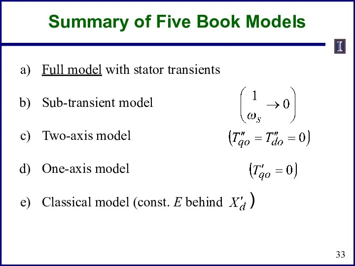
Full model with stator transients
Sub-transient model
Two-axis model
One-axis model
Classical model (const. E
Full model with stator transients
Sub-transient model
Two-axis model
One-axis model
Classical model (const. E
Damping Torques
Friction and windage
Usually small
Stator currents (load)
Usually represented in the load
Damping Torques
Friction and windage
Usually small
Stator currents (load)
Usually represented in the load
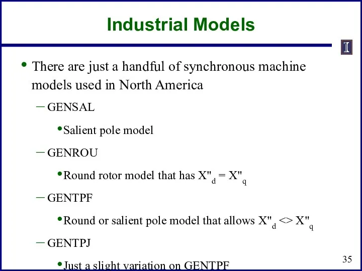
Industrial Models
There are just a handful of synchronous machine models used
Industrial Models
There are just a handful of synchronous machine models used
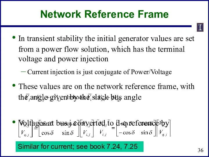
Network Reference Frame
In transient stability the initial generator values are set
Network Reference Frame
In transient stability the initial generator values are set
Network Reference Frame
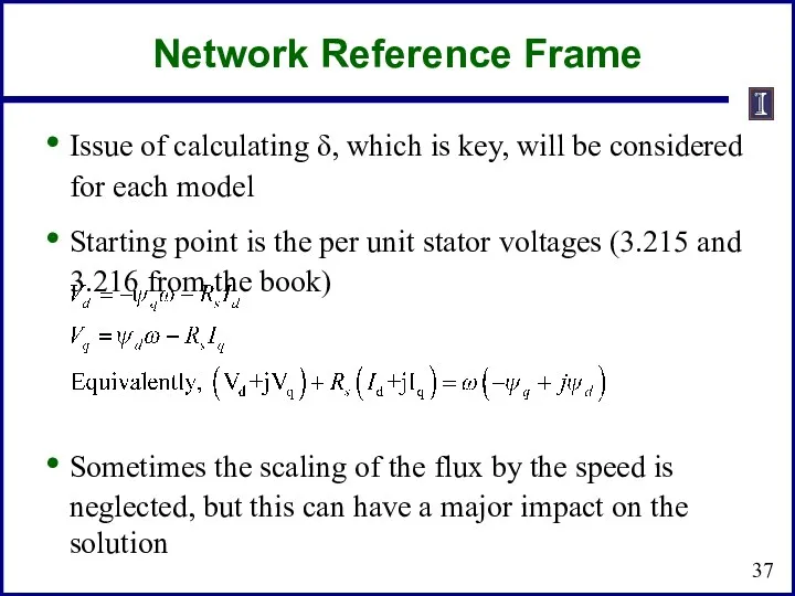
Issue of calculating δ, which is key, will be
Network Reference Frame
Issue of calculating δ, which is key, will be
Two-Axis Model
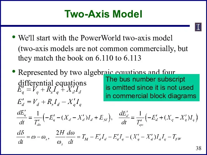
We'll start with the PowerWorld two-axis model (two-axis models are
Two-Axis Model
We'll start with the PowerWorld two-axis model (two-axis models are
Two-Axis Model
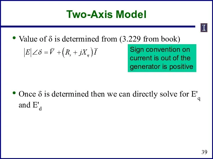
Value of δ is determined from (3.229 from book)
Once δ
Two-Axis Model
Value of δ is determined from (3.229 from book)
Once δ
Example (Used for All Models)
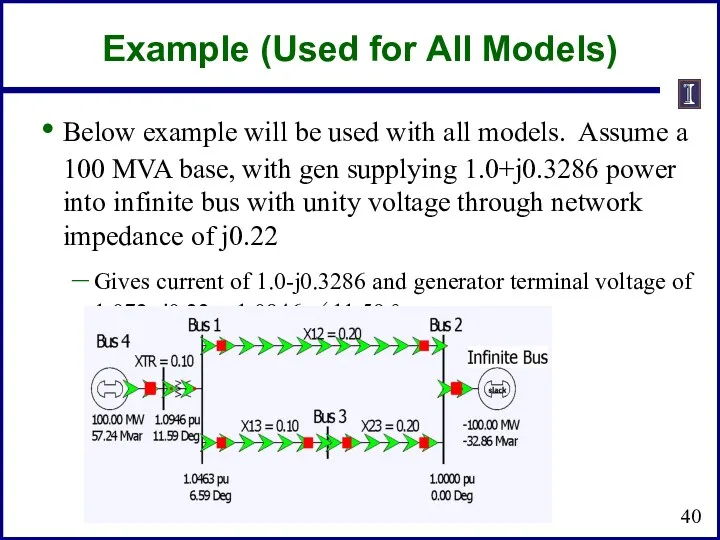
Below example will be used with all
Example (Used for All Models)
Below example will be used with all
Two-Axis Example
For the two-axis model assume H = 3.0 per unit-seconds,
Two-Axis Example
For the two-axis model assume H = 3.0 per unit-seconds,
Two-Axis Example
And
Saved as case B4_TwoAxis
Two-Axis Example
And
Saved as case B4_TwoAxis
Subtransient Models
The two-axis model is a transient model
Essentially all commercial studies
Subtransient Models
The two-axis model is a transient model
Essentially all commercial studies
Subtransient Models
Usually represented by a Norton Injection with
May also be shown
Subtransient Models
Usually represented by a Norton Injection with
May also be shown
GENSAL
The GENSAL model has been widely used to model salient pole
GENSAL
The GENSAL model has been widely used to model salient pole
GENSAL Block Diagram (PSLF)
A quadratic saturation function is used. For
initialization
GENSAL Block Diagram (PSLF)
A quadratic saturation function is used. For initialization
GENSAL Initialization
To initialize this model
Use S(1.0) and S(1.2) to solve
GENSAL Initialization
To initialize this model
Use S(1.0) and S(1.2) to solve
GENSAL Example
Assume same system as before, but with the generator parameters
GENSAL Example
Assume same system as before, but with the generator parameters
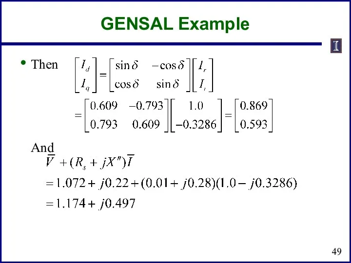
GENSAL Example
Then
And
GENSAL Example
Then
And
GENSAL Example
Giving the initial fluxes (with ω = 1.0)
To get the
GENSAL Example
Giving the initial fluxes (with ω = 1.0)
To get the
 Jobs and Professions
 The present simple tense (простое настоящее время). 5 класс
 Диалектные особенности английского языка
 Present Continuous Tense
 Article format
 The 10 Golden Rules of Customer Service
 Daily routines and freetime activities
 How do you like
 The theory of functional styles. Lecture 8
 Структура английского предложения
 Lecture 6. Word-building (part 2 )
 Письмо другу
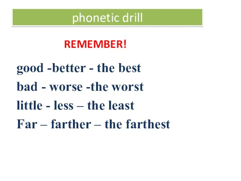 Phonetic drill. Complete the sentences and use a superlative form
 Today is the … of ……
 Comparative characteristics of cuisines British and Italian cuisine
 Past tenses
 My friend-animal
 Future in the past
 Module Сеlebrations Lesson 1 f English in Use
 Talking on family matters
 What can we do to save the Earht?
 Household chores
 Будущее простое время
 English for academic purposes (lesson 2)
 English professional
 Аdvertising
 Spotlight 3 unit 15a days of the week
 Welcome to Belarus