- HММ, поиск генов и профилей

Содержание
- 2. Поиск генов
- 3. Jan 23, 2003 Computational Gene Finding Gene Structure
- 4. What is it about genes that we can measure (and model)? Most of our knowledge is
- 5. Статистика кодирующей последовательности Неравное использование кодонов в кодирующих областях – универсальная характеристика геномов. Неравное использование аминокислот
- 6. An Example of Coding Statistics
- 7. Codon Adaptation Index (CAI) the geometric mean of the weight associated to each codon over the
- 8. CAI Example: Counts per 1000 codons
- 9. Splice signals (mice): GT , AG
- 10. HMMs and Prokaryotics Gene Structure Nucleotides {A,C,G,T} are the observables Different states generate nucleotides at different
- 11. Parse For a given sequence, a parse is an assignment of gene structure to that sequence.
- 12. The HMM Matrixes: Φ and H xm(i) = probability of being in state m at position
- 13. A eukaryotic gene This is the human p53 tumor suppressor gene on chromosome 17. Genscan is
- 14. A eukaryotic gene 3’ untranslated region Final exon Initial exon Introns Internal exons This particular gene
- 15. An Intron 3’ splice site 5’ splice site revcomp(CT)=AG revcomp(AC)=GT GT: signals start of intron AG:
- 16. Signals vs contents In gene finding, a small pattern within the genomic DNA is referred to
- 17. Prior knowledge We want to build a probabilistic model of a gene that incorporates our prior
- 18. Prior knowledge The translated region must have a length that is a multiple of 3. Some
- 19. Цепи Маркова высокого порядка k th-order Markov model bases the probability of an event on the
- 20. Цепи Маркова высокого порядка Advantages: Easy to train. Count frequencies of (k+1)-mers in training data. Easy
- 21. Genscan Example Uses explicit state duration HMM to model gene structure (different length distributions for exons)
- 22. E0 E1 E2 E2 E1 E0 N P Eterm P Einit polyA 5’ UTR I0 I1
- 23. http://nar.oxfordjournals.org/content/26/4/1107
- 24. GeneMark Borodovsky & McIninch, Comp. Chem 17, 1993. Uses 5th-order Markov model. Model is 3-periodic, i.e.,
- 25. Interpolated Markov Models (IMM) Introduced in Glimmer 1.0 Salzberg, Delcher, Kasif & White, NAR 26, 1998.
- 26. Real IMMs Model has additional probabilities, λ, that determine which parts of the context to use.
- 27. Real IMMs Result is a linear combination of different Markov orders: where Can view this as
- 28. IMMs vs Fixed-Order Models Performance IMM generally should do at least as well as a fixed-order
- 29. GLIMMER-HMM Nth-order interpolated Markov models (IMM) (N=8)
- 30. General Things to Remember about (Protein-coding) Gene Prediction Software It is, in general, organism-specific It works
- 31. Профильные HMM Profile HMM Берем множественное выравнивание и делаем из него статистическую модель.
- 33. Profile HMMs Моделирует семейство последовательностей Вычисляется из множественного выравнивания семейства Вероятности переходов состояний и испускания данных
- 34. Строим модель: состояния совпадения (Match States) Если нам нужно выполнить выравнивание без пропусков, то мы можем
- 35. Состояния вставки Insertion States Во множественном выравнивании часто встречаются колонки, являющиеся пропусками в большинстве последовательностях, но
- 36. Состояние делиции Deletion States Делициями во множественном выравнивании называют позиции, в которых большинство последовательностей имеют аминокислоты,
- 37. Profile HMMs Существует также переход из состоянии вставки в состояние делиции, но такие переходы считаются маловероятными,
- 38. Profile HMMs: Example Note: These sequences could lead to other paths.
- 39. Pfam “A comprehensive collection of protein domains and families, with a range of well-established uses including
- 41. A Profile HMM Example This is a section of a repeated sequence in Bacillus megaterium. 15
- 42. Cоздание модели Что называть вставками, что делициями? >50% пропусков -> вставка делиция 9 последовательностей имеют разрыв
- 43. More Set Up Колонки 2 и 3- состояния делиции, но в других последовательностях – состояния совпадения.
- 44. Параметризация Какие параметры нам нужны? Эмиссионные: В каждом состояние надо задать вероятности эмиссии для всех 4
- 45. Эмиссионные вероятности Фоновый уровень (вероятности оснований, если бы они были выбраны случайным образом) Используются для состояний
- 46. Эмиссионные псевдочастоты The simplest way to do pseudocounts is the Laplace method: adding 1 to the
- 47. Частоты переходов Всего 225 переходов, и только 9 M->D. P(M->D) = 9/225 = 0.040. Для D->D,
- 48. Специфические переходы Колонки вставок и делиций. Колонка 2 содержит 1 M->D и14 M->M. Need to add
- 49. Emission Probability Tables
- 50. Transitions
- 51. Scoring a Sequence Whew! We have now estimated parameters for all transitions and emissions. Scoring a
- 52. Scoring GGGGAAAAACGTATT Base 1 is G. To start the global model off, we are going to
- 53. More Scoring Base 3 is also a G. M2->M3 has 0.420 probability and 0.464 chance of
- 54. Still More Scoring GGG GAAAA ACGTATT The next several bases are easy. Since the probability of
- 55. Yet More At this point we have emitted positions 1- 8, and the most probable path
- 56. Yet Still More At this point we have emitted positions 1- 8, and the most probable
- 57. To the End… Our path so far: M1->M2->D->M4->M5->M6->M7->M8->M9->M10->I GGG GAAAAAC GTATT From the insert state we
- 58. Final probability We need to know what the probability would be for the random model, with
- 59. Profile Hidden Markov Models Вычисление веса последовательности по профильным HMM Имея профильную HMM, любой путь по
- 60. Profile Hidden Markov Models Вычисление веса последовательности по профильным HMM Алгоритм Витерби: Имея исходную последовательность, мы
- 62. Скачать презентацию
 α-аминокислоты. Пептиды. Белки. (Лекция 5)
 Клиническая биохимия азотистого обмена. (Лекция 7)
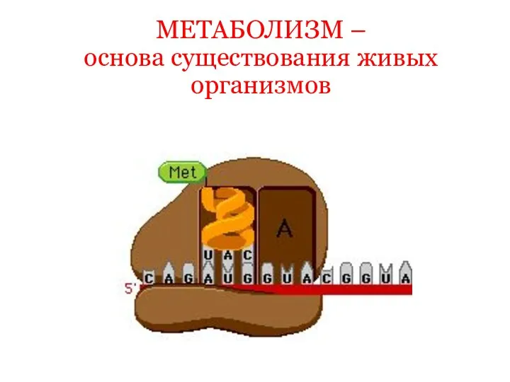 Метаболизм – основа существования живых организмов
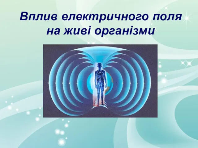 Вплив електричного поля на живі організми
 Skin receptors
 Животные Мурманской области
 Возникновение и развитие эволюционных представлений. Эволюционная теория
 Биологические особенности и технология выращивания капусты кочанной
 Этапы развития головного мозга
 презентация по теме:Закономерности наследования признаков, установленных Г.Менделем, урок биологии в 9 классе
 Мейоз. Механизм мейоза
 Домашний доктор
 Большие кошки. Гепард
 Презентация Экологические факторы.
 Голосеменные растения
 Суспільні комахи
 Морфологические изменения в хрусталике при катаракте
 Инструкция по обслуживанию и уходу за зеленой стеной
 Квіткові рослини. Розмноження квіткових рослин
 Е-Планер. Эмоции и чувства. 4 класс
 Комнатные растения и уход за ними
 Вегетативное размножение растений
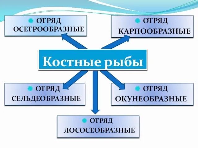 Костные рыбы
 Vitamins. Classification
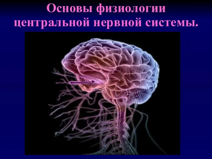 Основы физиологии центральной нервной системы
 Микология. Классификация и морфология грибов
 Жизненные циклы растений
 Строение прокариотической и эукариотической клеток