- Aggregate demand and aggregate supply analysis

Содержание
- 2. Learning Objectives Understand what happens during business cycles and their relationship to long-run economic growth. Discuss
- 3. Learning Objectives Use the aggregate demand and aggregate supply model to illustrate the difference between short-run
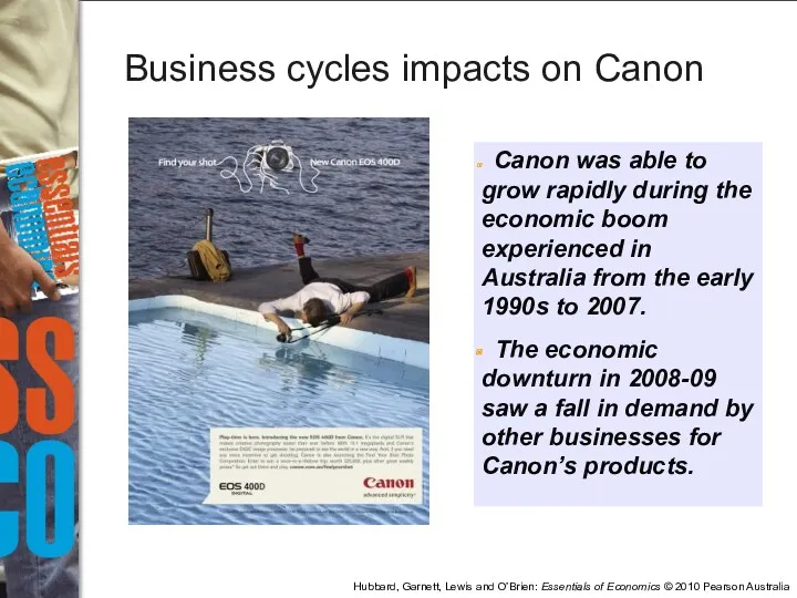
- 4. Business cycles impacts on Canon Canon was able to grow rapidly during the economic boom experienced
- 5. Business cycle: Alternating periods of economic expansion and economic recession. The expansion phase Production, employment and
- 6. Recession: A significant decline in activity spread across the economy, lasting more than a few months,
- 7. Movements in real GDP, Australia, 1980 – 2007: Figure 13.1 Source: Australian Bureau of Statistics (2008),
- 8. What happens during a business cycle? Each business cycle is different, however all share some similarities.
- 9. What happens during a business cycle? The effect of the business cycle on car sales. Consumer
- 10. The effect of the business cycle on new car sales, Australia, 1994 – 2007: Figure 13.2
- 11. What happens during a business cycle? The impact of a recession on the inflation rate. During
- 12. The impact of a recession on the inflation rate, Australia: Figure 13.3 Source: Reserve Bank of
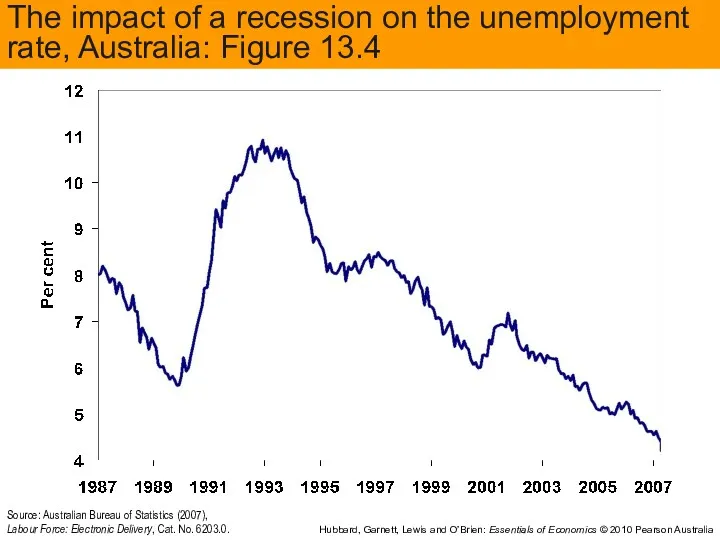
- 13. What happens during a business cycle? The impact of a recession on the unemployment rate. Recessions
- 14. The impact of a recession on the unemployment rate, Australia: Figure 13.4 Source: Australian Bureau of
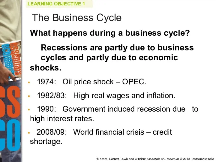
- 15. What happens during a business cycle? Recessions are partly due to business cycles and partly due
- 16. Fluctuations in real GDP, Australia, 1960-2007: Figure 13.5 Source: Australian Bureau of Statistics (2007), Australian National
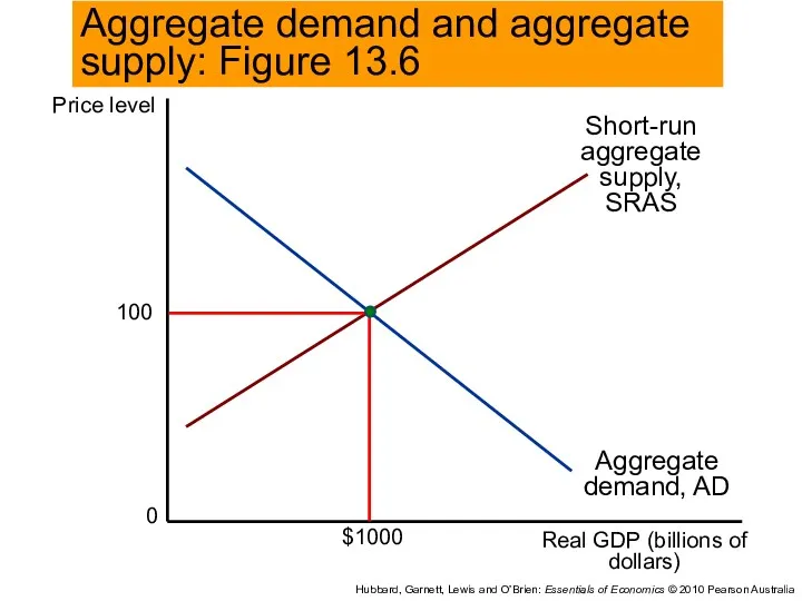
- 17. Aggregate demand and aggregate supply model: A model that explains short-run fluctuations in real GDP and
- 18. Aggregate demand curve (AD): A curve showing the relationship between the price level and the quantity
- 19. Price level Real GDP (billions of dollars) 0 $1000 Hubbard, Garnett, Lewis and O’Brien: Essentials of
- 20. Why is the aggregate demand curve downward sloping? The wealth effect How a change in the
- 21. Shifts in the aggregate demand curve versus movements along it. The AD curve shows the relationship
- 22. The variables that shift the aggregate demand curve: Changes in government policies. Examples: taxes; government purchases.
- 23. The effect of exchange rates on sales During some years, the falling value of the Australian
- 24. Determinants of Aggregate Demand Explain whether each of the following will cause a movement along or
- 25. Determinants of Aggregate Demand a) Rising interest rates cause a drop in consumer optimism as households
- 26. STEP 1: Review the material. This question is intended to help differentiate between events that will
- 27. STEP 2: Answering (a): Households become pessimistic about the future. In order to ensure they can
- 28. Aggregate quantity demanded will decrease as households spend less in order to contribute more to their
- 29. The long-run aggregate supply curve (LRAS): A curve showing the relationship in the long run between
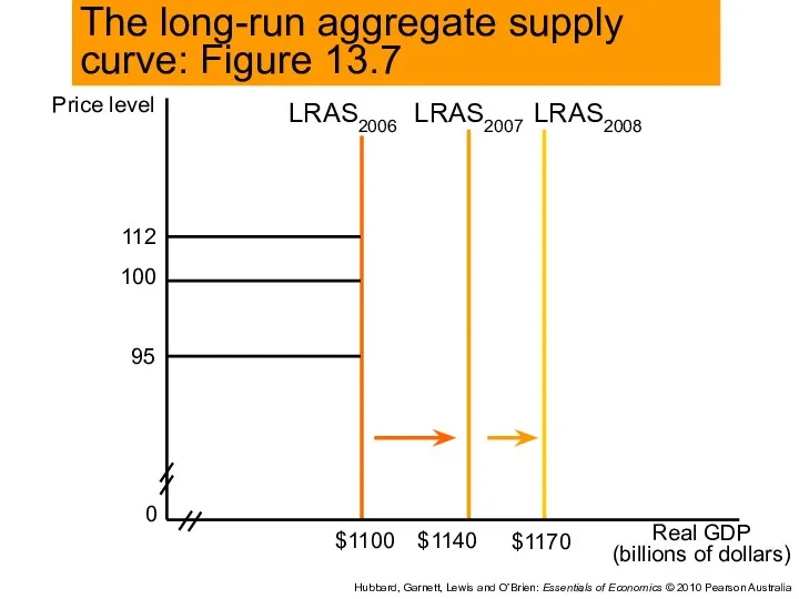
- 30. Shifts in the long-run aggregate supply curve. The LRAS curve shifts because potential real GDP increases
- 31. Price level Real GDP (billions of dollars) 0 $1100 Hubbard, Garnett, Lewis and O’Brien: Essentials of
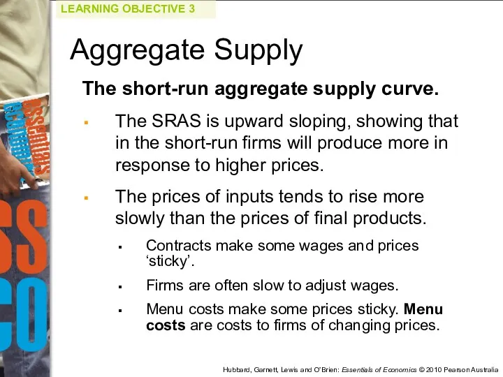
- 32. The short-run aggregate supply curve. The SRAS is upward sloping, showing that in the short-run firms
- 33. Shifts in the short-run aggregate supply curve versus movements along it. The SRAS curve shows the
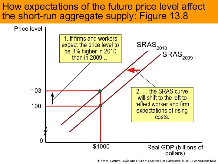
- 34. Variables that shift the SRAS curve. Expected changes in the future price level. Adjustments of workers
- 35. Price level Real GDP (billions of dollars) 0 $1000 Hubbard, Garnett, Lewis and O’Brien: Essentials of
- 36. Variables that shift the short-run and the long-run aggregate supply curves. Increases in the labour force
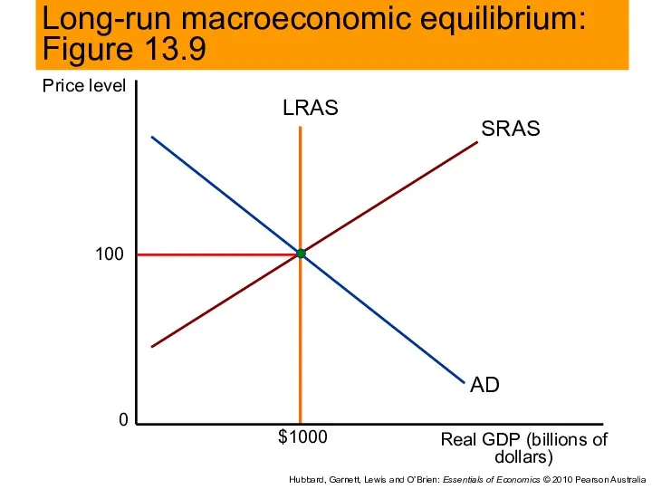
- 37. In long-run equilibrium, the aggregate demand and short-run aggregate supply curves intersect at a point along
- 38. Price level Real GDP (billions of dollars) 0 $1000 Hubbard, Garnett, Lewis and O’Brien: Essentials of
- 39. Recessions, expansions and supply shocks. The following analysis of the aggregate demand and aggregate supply model
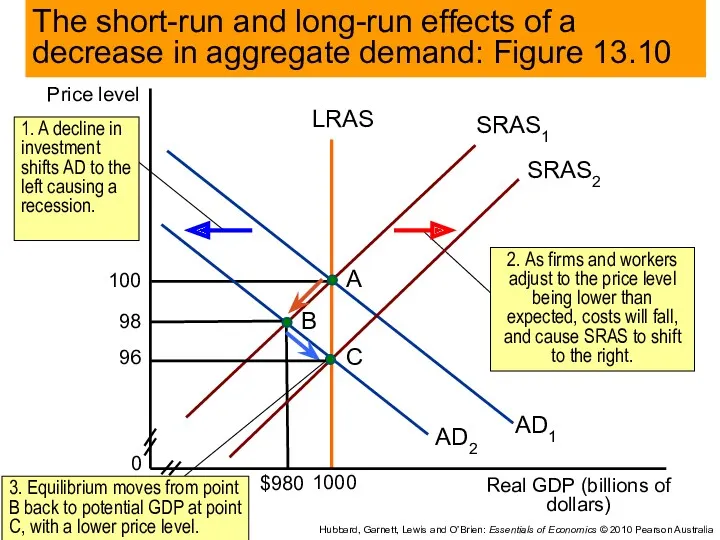
- 40. Recession The short-run effect of a decline in aggregate demand. AD curve shifts left, and real
- 41. Price level Real GDP (billions of dollars) 0 1000 Hubbard, Garnett, Lewis and O’Brien: Essentials of
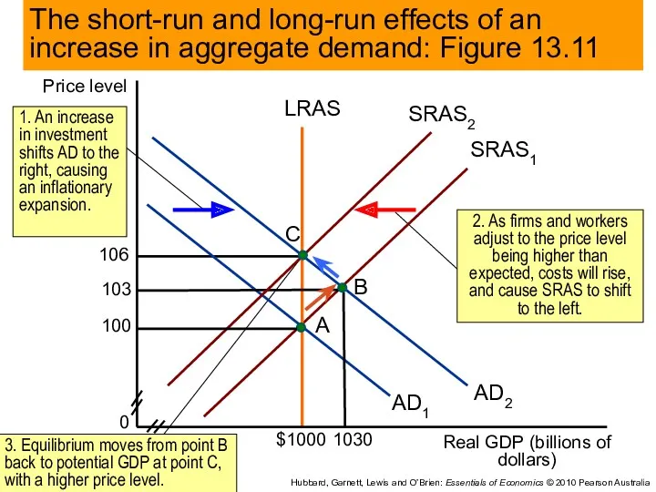
- 42. Expansion The short-run effect of an increase in aggregate demand. AD curve shifts right, real GDP
- 43. Price level Real GDP (billions of dollars) 0 $1000 Hubbard, Garnett, Lewis and O’Brien: Essentials of
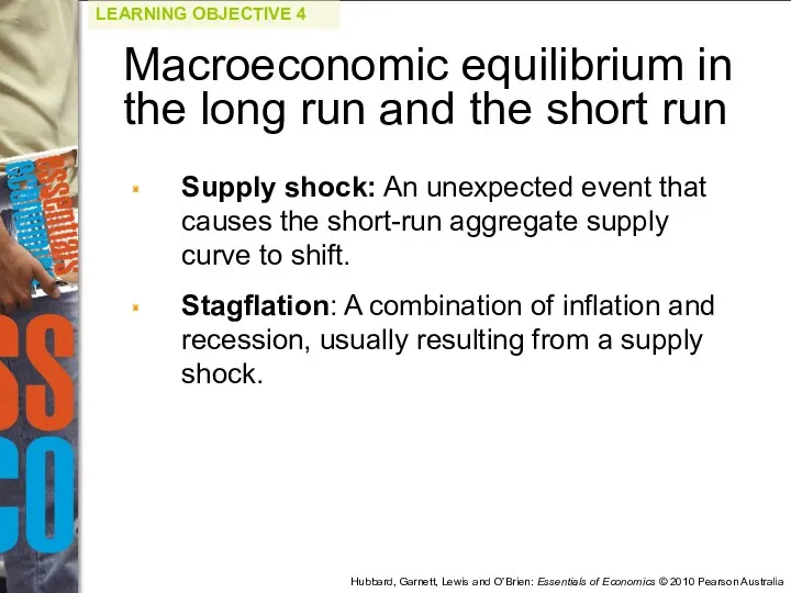
- 44. Supply shock: An unexpected event that causes the short-run aggregate supply curve to shift. Stagflation: A
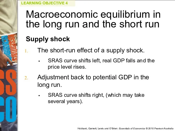
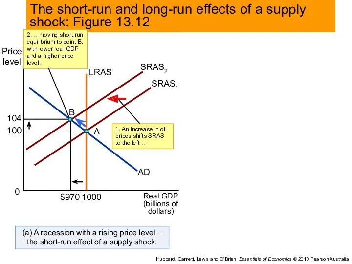
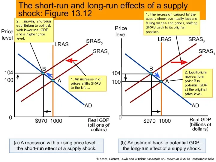
- 45. Supply shock The short-run effect of a supply shock. SRAS curve shifts left, real GDP falls
- 46. (b) Adjustment back to potential GDP – the long-run effect of a supply shock. 0 (a)
- 47. (b) Adjustment back to potential GDP – the long-run effect of a supply shock. 0 (a)
- 48. Using the Aggregate Demand Aggregate Supply model. Assume the economy is initially in equilibrium with long-run
- 49. STEP 1: Review the chapter material. The basic equilibrium model is explained in the section on
- 50. The price level is now higher than workers and firms had expected. As workers and firms
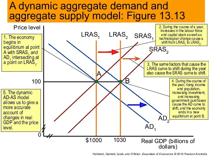
- 51. A dynamic aggregate demand and aggregate supply model can be created by making three changes to
- 52. Price level Real GDP (billions of dollars) 0 $1000 Hubbard, Garnett, Lewis and O’Brien: Essentials of
- 53. Price level Real GDP (billions of dollars) 0 $1000 Hubbard, Garnett, Lewis and O’Brien: Essentials of
- 54. Does rising productivity growth reduce employment? New technology and equipment increases labour productivity. MAKING THE CONNECTION
- 55. JB Hi-Fi reports sales up 36% and net profit after tax up 56%. An Inside Look
- 56. An Inside Look Figure 1: Australian economic expansion between 2002 and 2007 Hubbard, Garnett, Lewis and
- 57. Key Terms Aggregate demand and aggregate supply model Aggregate demand curve (AD) Business cycle Long-run aggregate
- 58. At various times, the Australian dollar increases in value against the US dollar and other major
- 59. Q1. From a trough to a peak, the economy goes through: a. The recession phase of
- 60. Q1. From a trough to a peak, the economy goes through: a. The recession phase of
- 61. Q2. During the early stages of a recovery: a. Firms usually rush to hire new employees
- 62. Q2. During the early stages of a recovery: a. Firms usually rush to hire new employees
- 63. Q3. The aggregate demand curve shows the relationship between the price level and the quantity of
- 64. Q3. The aggregate demand curve shows the relationship between the price level and the quantity of
- 65. Q4. Which of the following factors do not cause the aggregate demand curve to shift? a.
- 66. Q4. Which of the following factors do not cause the aggregate demand curve to shift? a.
- 67. Q5. How can government policies shift the aggregate demand curve to the right? a. By increasing
- 68. Q5. How can government policies shift the aggregate demand curve to the right? a. By increasing
- 69. Q6. Which of the following statements is true? a. In the long run, increases in the
- 70. Q6. Which of the following statements is true? a. In the long run, increases in the
- 71. Q7. Which of the following would shift both the short-run and the long-run aggregate supply curves?
- 72. Q7. Which of the following would shift both the short-run and the long-run aggregate supply curves?
- 73. Q8. Which of the following is usually the cause of stagflation? a. Reductions in government spending.
- 74. Q8. Which of the following is usually the cause of stagflation? a. Reductions in government spending.
- 75. Aggregate Expenditure Model: A macroeconomic model that focuses on the relationship between total spending and real
- 76. An example of a 45° line diagram: Figure 13A.1 Hubbard, Garnett, Lewis and O’Brien: Essentials of
- 77. Aggregate Expenditure (AE): The total amount of spending in the economy: the sum of consumption (C),
- 78. Using the 45° line diagram to illustrate macroeconomic equilibrium. The 45° line measures real national income
- 79. The relationship between planned aggregate expenditure and GDP on a 45° line diagram: Figure 13A.2 Hubbard,
- 80. Consumption function: The relationship between consumption spending and disposable income. The consumption function intersects the vertical
- 81. Macroeconomic equilibrium on the 45° line diagram: Figure 13A.3 Hubbard, Garnett, Lewis and O’Brien: Essentials of
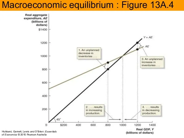
- 82. The AE line intersects the 45° line at equilibrium real GDP. At points above the 45°
- 83. Macroeconomic equilibrium : Figure 13A.4 Hubbard, Garnett, Lewis and O’Brien: Essentials of Economics © 2010 Pearson
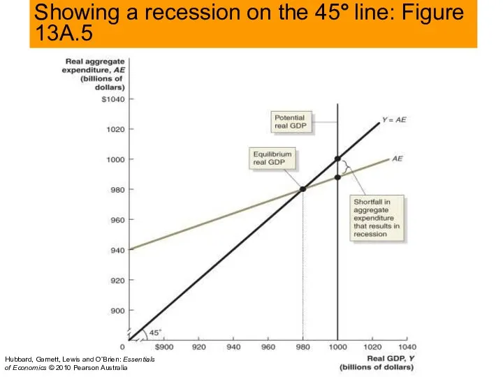
- 84. Showing a recession on the 45° line diagram Macroeconomic equilibrium can occur at any point on
- 85. Showing a recession on the 45° line: Figure 13A.5 Hubbard, Garnett, Lewis and O’Brien: Essentials of
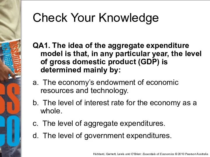
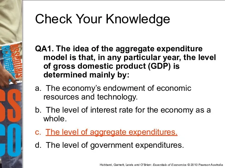
- 86. QA1. The idea of the aggregate expenditure model is that, in any particular year, the level
- 87. QA1. The idea of the aggregate expenditure model is that, in any particular year, the level
- 88. QA2. Which of the following statements is correct? Actual investment and planned investment are always the
- 90. Скачать презентацию
Learning Objectives
Understand what happens during business cycles and their relationship to
Learning Objectives
Understand what happens during business cycles and their relationship to
Learning Objectives
Use the aggregate demand and aggregate supply model to illustrate
Learning Objectives
Use the aggregate demand and aggregate supply model to illustrate
Business cycles impacts on Canon
Canon was able to grow rapidly
Business cycles impacts on Canon
Canon was able to grow rapidly
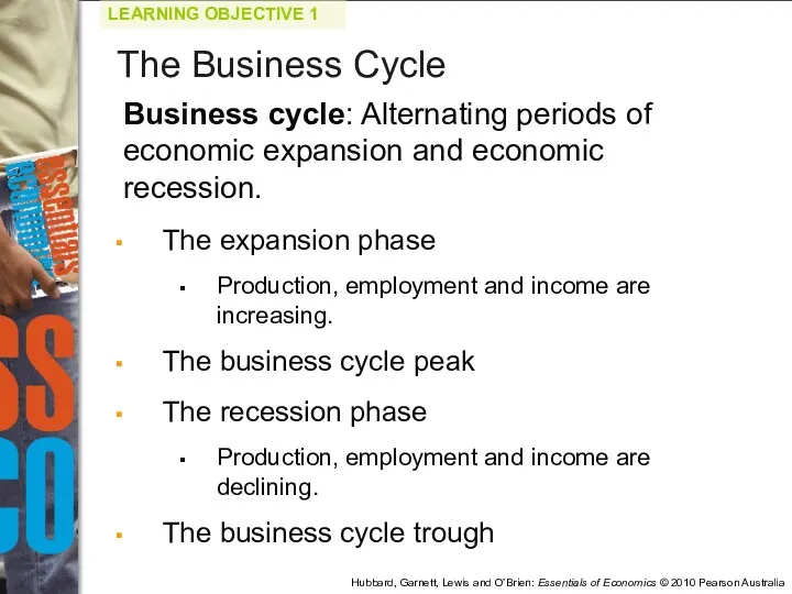
Business cycle: Alternating periods of economic expansion and economic recession.
The
Business cycle: Alternating periods of economic expansion and economic recession.
The
Recession: A significant decline in activity spread across the economy, lasting
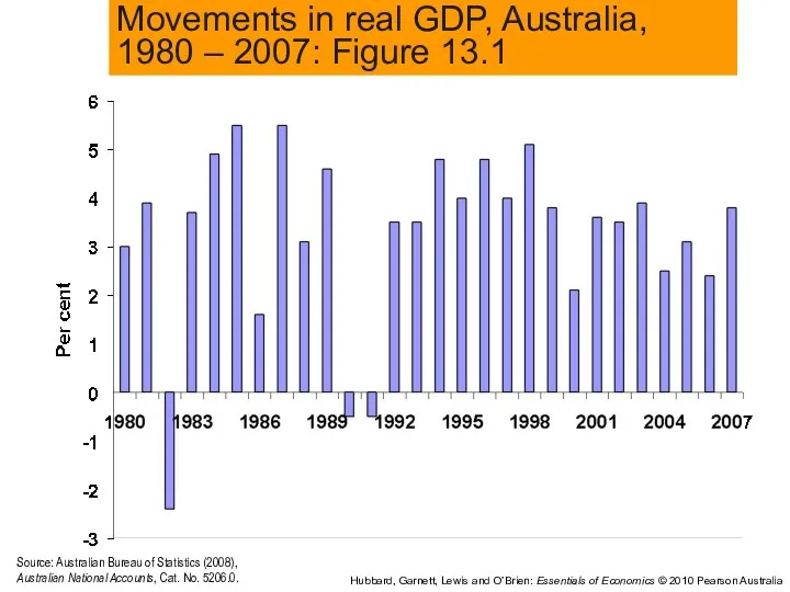
Movements in real GDP, Australia,
1980 – 2007: Figure 13.1
Source: Australian
Movements in real GDP, Australia,
1980 – 2007: Figure 13.1
Source: Australian
What happens during a business cycle?
Each business cycle is
What happens during a business cycle?
Each business cycle is
What happens during a business cycle?
The effect of the
What happens during a business cycle?
The effect of the
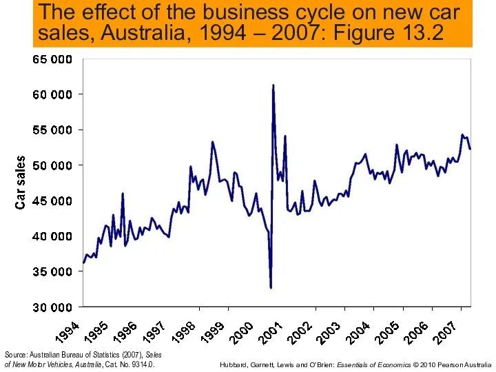
The effect of the business cycle on new car sales, Australia,
The effect of the business cycle on new car sales, Australia,
What happens during a business cycle?
The impact of a recession
What happens during a business cycle?
The impact of a recession
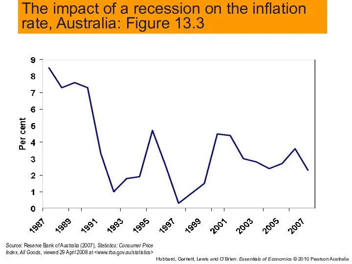
The impact of a recession on the inflation rate, Australia: Figure
The impact of a recession on the inflation rate, Australia: Figure
What happens during a business cycle?
The impact of a recession
What happens during a business cycle?
The impact of a recession
The impact of a recession on the unemployment rate, Australia: Figure
The impact of a recession on the unemployment rate, Australia: Figure
What happens during a business cycle?
Recessions are partly due to
What happens during a business cycle?
Recessions are partly due to

Fluctuations in real GDP, Australia,
1960-2007: Figure 13.5
Source: Australian Bureau of
Fluctuations in real GDP, Australia,
1960-2007: Figure 13.5
Source: Australian Bureau of
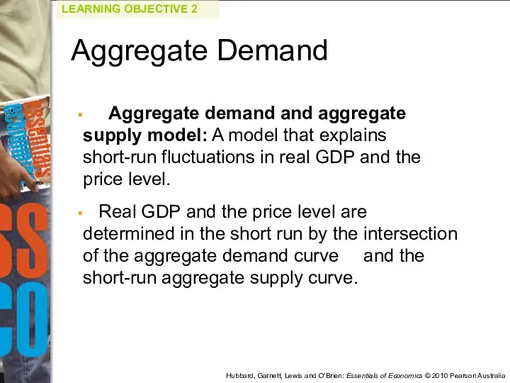
Aggregate demand and aggregate supply model: A model that explains
Aggregate demand and aggregate supply model: A model that explains
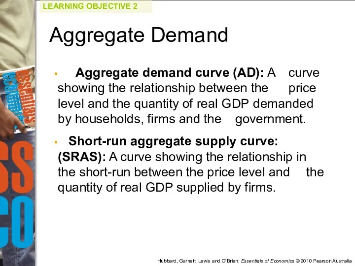
Aggregate demand curve (AD): A curve showing the relationship between the
Aggregate demand curve (AD): A curve showing the relationship between the
Price level
Real GDP (billions of dollars)
0
$1000
Hubbard, Garnett, Lewis and O’Brien: Essentials
Price level
Real GDP (billions of dollars)
0
$1000
Hubbard, Garnett, Lewis and O’Brien: Essentials
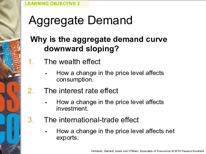
Why is the aggregate demand curve downward sloping?
The wealth effect
How
Why is the aggregate demand curve downward sloping?
The wealth effect
How
Shifts in the aggregate demand curve versus movements along it.
The AD
Shifts in the aggregate demand curve versus movements along it.
The AD
The variables that shift the aggregate demand curve:
Changes in government
The variables that shift the aggregate demand curve:
Changes in government

The effect of exchange rates on sales
During some years, the falling
The effect of exchange rates on sales
During some years, the falling
Determinants of Aggregate Demand
Explain whether each of the following will
Determinants of Aggregate Demand
Explain whether each of the following will
Determinants of Aggregate Demand
a) Rising interest rates cause a drop
Determinants of Aggregate Demand
a) Rising interest rates cause a drop
STEP 1: Review the material. This question is intended to
STEP 1: Review the material. This question is intended to
STEP 2: Answering (a): Households become pessimistic about the future.
STEP 2: Answering (a): Households become pessimistic about the future.
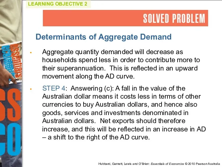
Aggregate quantity demanded will decrease as households spend less in
Aggregate quantity demanded will decrease as households spend less in
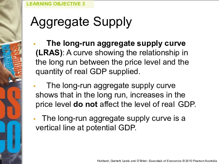
The long-run aggregate supply curve (LRAS): A curve showing the
The long-run aggregate supply curve (LRAS): A curve showing the
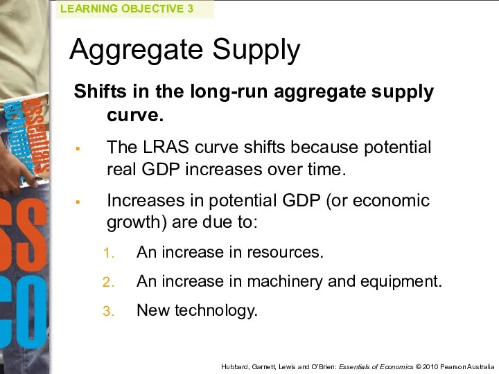
Shifts in the long-run aggregate supply curve.
The LRAS curve shifts because
Shifts in the long-run aggregate supply curve.
The LRAS curve shifts because
Price level
Real GDP (billions of dollars)
0
$1100
Hubbard, Garnett, Lewis and O’Brien: Essentials
Price level
Real GDP (billions of dollars)
0
$1100
Hubbard, Garnett, Lewis and O’Brien: Essentials
The short-run aggregate supply curve.
The SRAS is upward sloping, showing that
The short-run aggregate supply curve.
The SRAS is upward sloping, showing that
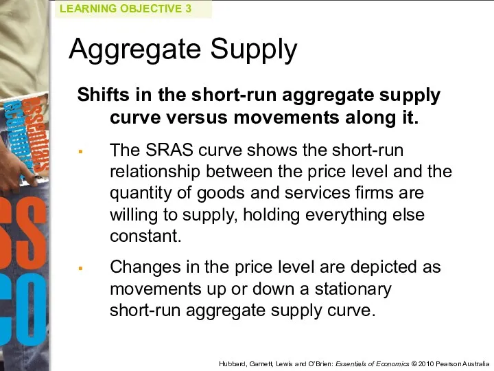
Shifts in the short-run aggregate supply curve versus movements along it.
The
Shifts in the short-run aggregate supply curve versus movements along it.
The
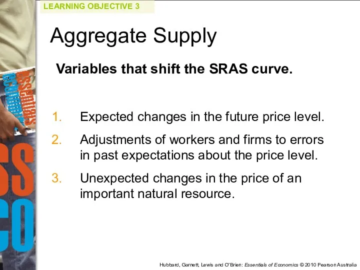
Variables that shift the SRAS curve.
Expected changes in the future price
Variables that shift the SRAS curve.
Expected changes in the future price
Price level
Real GDP (billions of dollars)
0
$1000
Hubbard, Garnett, Lewis and O’Brien: Essentials
Price level
Real GDP (billions of dollars)
0
$1000
Hubbard, Garnett, Lewis and O’Brien: Essentials
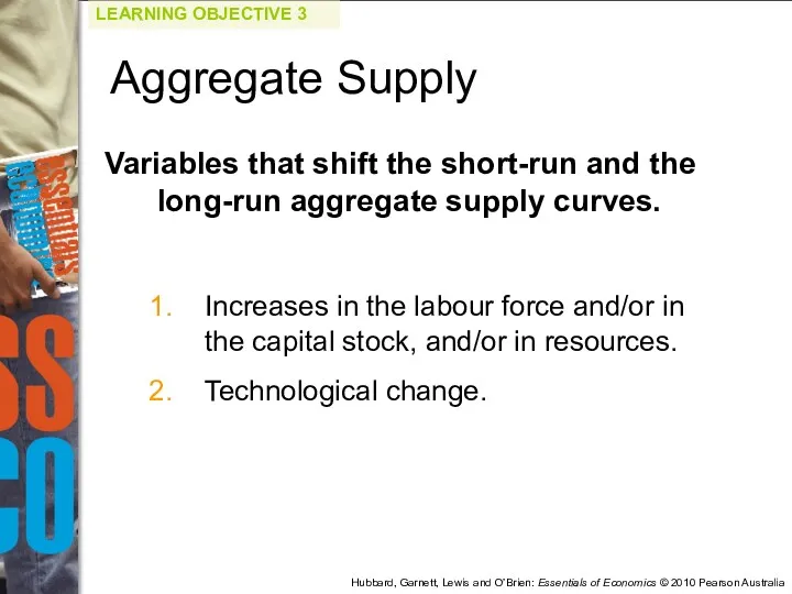
Variables that shift the short-run and the long-run aggregate supply curves.
Increases
Variables that shift the short-run and the long-run aggregate supply curves.
Increases
In long-run equilibrium, the aggregate demand and short-run aggregate supply
In long-run equilibrium, the aggregate demand and short-run aggregate supply
Price level
Real GDP (billions of dollars)
0
$1000
Hubbard, Garnett, Lewis and O’Brien: Essentials
Price level
Real GDP (billions of dollars)
0
$1000
Hubbard, Garnett, Lewis and O’Brien: Essentials
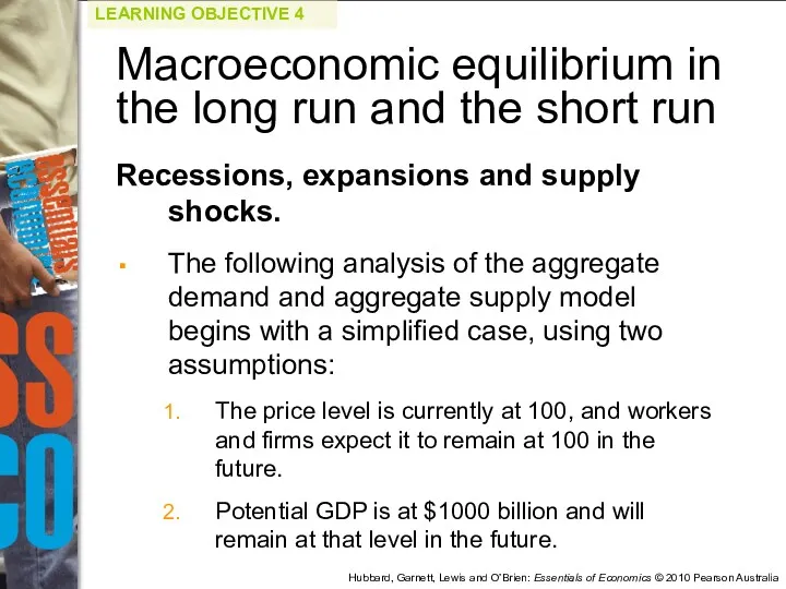
Recessions, expansions and supply shocks.
The following analysis of the aggregate
Recessions, expansions and supply shocks.
The following analysis of the aggregate
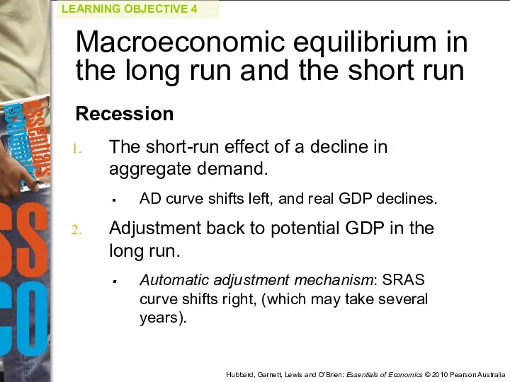
Recession
The short-run effect of a decline in aggregate demand.
AD curve shifts
Recession
The short-run effect of a decline in aggregate demand.
AD curve shifts
Price level
Real GDP (billions of dollars)
0
1000
Hubbard, Garnett, Lewis and O’Brien: Essentials
Price level
Real GDP (billions of dollars)
0
1000
Hubbard, Garnett, Lewis and O’Brien: Essentials
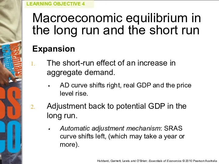
Expansion
The short-run effect of an increase in aggregate demand.
AD curve shifts
Expansion
The short-run effect of an increase in aggregate demand.
AD curve shifts
Price level
Real GDP (billions of dollars)
0
$1000
Hubbard, Garnett, Lewis and O’Brien: Essentials
Price level
Real GDP (billions of dollars)
0
$1000
Hubbard, Garnett, Lewis and O’Brien: Essentials
Supply shock: An unexpected event that causes the short-run aggregate supply
Supply shock: An unexpected event that causes the short-run aggregate supply
Supply shock
The short-run effect of a supply shock.
SRAS curve shifts left,
Supply shock
The short-run effect of a supply shock.
SRAS curve shifts left,
(b) Adjustment back to potential GDP – the long-run effect of
(b) Adjustment back to potential GDP – the long-run effect of
(b) Adjustment back to potential GDP – the long-run effect of
(b) Adjustment back to potential GDP – the long-run effect of
Using the Aggregate Demand Aggregate Supply model.
Assume the economy is
Using the Aggregate Demand Aggregate Supply model.
Assume the economy is
STEP 1: Review the chapter material. The basic equilibrium model
STEP 1: Review the chapter material. The basic equilibrium model
The price level is now higher than workers and firms
The price level is now higher than workers and firms
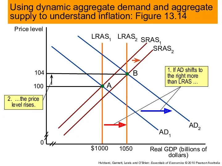
A dynamic aggregate demand and aggregate supply model can be created
A dynamic aggregate demand and aggregate supply model can be created
Price level
Real GDP (billions of dollars)
0
$1000
Hubbard, Garnett, Lewis and O’Brien: Essentials
Price level
Real GDP (billions of dollars)
0
$1000
Hubbard, Garnett, Lewis and O’Brien: Essentials
Price level
Real GDP (billions of dollars)
0
$1000
Hubbard, Garnett, Lewis and O’Brien: Essentials
Price level
Real GDP (billions of dollars)
0
$1000
Hubbard, Garnett, Lewis and O’Brien: Essentials

Does rising productivity growth reduce employment?
New technology and equipment increases labour
Does rising productivity growth reduce employment?
New technology and equipment increases labour
JB Hi-Fi reports sales up 36% and net profit after tax
JB Hi-Fi reports sales up 36% and net profit after tax

An Inside Look
Figure 1: Australian economic expansion between 2002 and 2007
Hubbard,
An Inside Look
Figure 1: Australian economic expansion between 2002 and 2007
Hubbard,
Key Terms
Aggregate demand and aggregate supply model
Aggregate demand curve (AD)
Business cycle
Long-run
Key Terms
Aggregate demand and aggregate supply model
Aggregate demand curve (AD)
Business cycle
Long-run

At various times, the Australian dollar increases in value against the
At various times, the Australian dollar increases in value against the
Q1. From a trough to a peak, the economy goes through:
a. The
Q1. From a trough to a peak, the economy goes through:
a. The
Q1. From a trough to a peak, the economy goes through:
a. The
Q1. From a trough to a peak, the economy goes through:
a. The
Q2. During the early stages of a recovery:
a. Firms usually rush to
Q2. During the early stages of a recovery:
a. Firms usually rush to
Q2. During the early stages of a recovery:
a. Firms usually rush
Q2. During the early stages of a recovery:
a. Firms usually rush
Q3. The aggregate demand curve shows the relationship between the price
Q3. The aggregate demand curve shows the relationship between the price
Q3. The aggregate demand curve shows the relationship between the price
Q3. The aggregate demand curve shows the relationship between the price
Q4. Which of the following factors do not cause the aggregate
Q4. Which of the following factors do not cause the aggregate
Q4. Which of the following factors do not cause the aggregate
Q4. Which of the following factors do not cause the aggregate
Q5. How can government policies shift the aggregate demand curve to
Q5. How can government policies shift the aggregate demand curve to
Q5. How can government policies shift the aggregate demand curve to
Q5. How can government policies shift the aggregate demand curve to
Q6. Which of the following statements is true?
a. In the long
Q6. Which of the following statements is true?
a. In the long
Q6. Which of the following statements is true?
a. In the long
Q6. Which of the following statements is true?
a. In the long
Q7. Which of the following would shift both the short-run and
Q7. Which of the following would shift both the short-run and
Q7. Which of the following would shift both the short-run and
Q7. Which of the following would shift both the short-run and
Q8. Which of the following is usually the cause of stagflation?
a.
Q8. Which of the following is usually the cause of stagflation?
a.
Q8. Which of the following is usually the cause of stagflation?
a.
Q8. Which of the following is usually the cause of stagflation?
a.
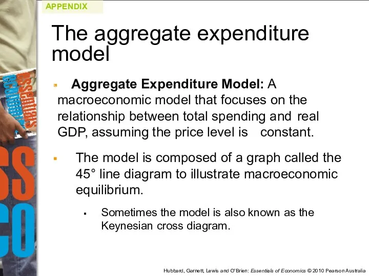
Aggregate Expenditure Model: A macroeconomic model that focuses on the
Aggregate Expenditure Model: A macroeconomic model that focuses on the
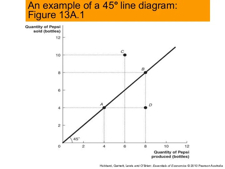
An example of a 45° line diagram: Figure 13A.1
Hubbard, Garnett, Lewis
An example of a 45° line diagram: Figure 13A.1
Hubbard, Garnett, Lewis
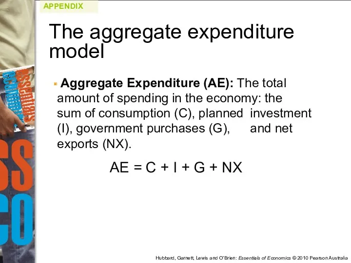
Aggregate Expenditure (AE): The total amount of spending in the
Aggregate Expenditure (AE): The total amount of spending in the
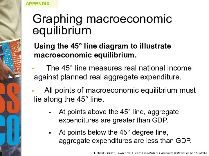
Using the 45° line diagram to illustrate macroeconomic equilibrium.
The 45°
Using the 45° line diagram to illustrate macroeconomic equilibrium.
The 45°
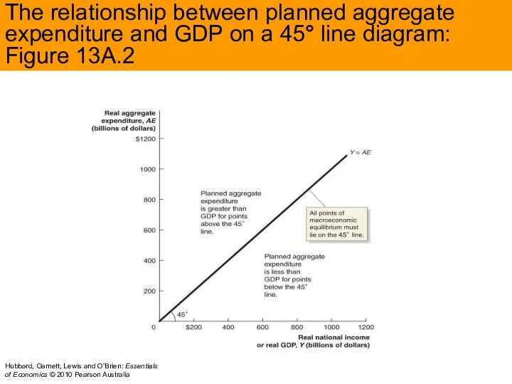
The relationship between planned aggregate expenditure and GDP on a 45°
The relationship between planned aggregate expenditure and GDP on a 45°
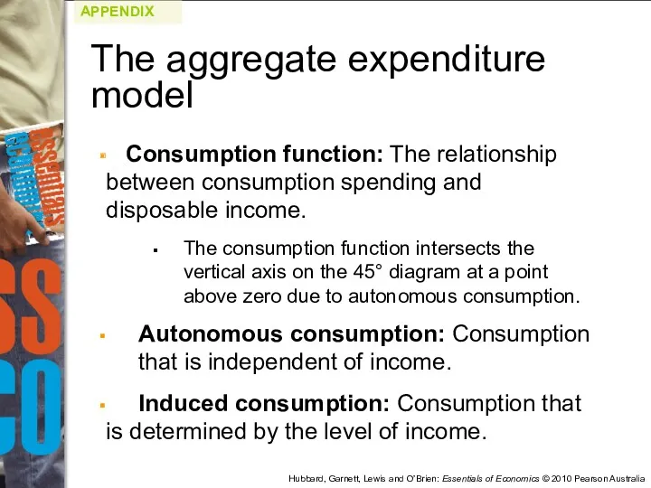
Consumption function: The relationship between consumption spending and disposable income.
The
Consumption function: The relationship between consumption spending and disposable income.
The
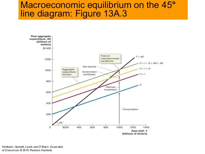
Macroeconomic equilibrium on the 45° line diagram: Figure 13A.3
Hubbard, Garnett, Lewis
Macroeconomic equilibrium on the 45° line diagram: Figure 13A.3
Hubbard, Garnett, Lewis
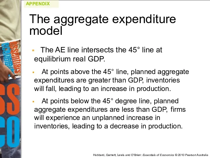
The AE line intersects the 45° line at equilibrium real
The AE line intersects the 45° line at equilibrium real
Macroeconomic equilibrium : Figure 13A.4
Hubbard, Garnett, Lewis and O’Brien: Essentials of
Macroeconomic equilibrium : Figure 13A.4
Hubbard, Garnett, Lewis and O’Brien: Essentials of
Showing a recession on the 45° line diagram
Macroeconomic equilibrium can
Showing a recession on the 45° line diagram
Macroeconomic equilibrium can
Showing a recession on the 45° line: Figure 13A.5
Hubbard, Garnett,
Showing a recession on the 45° line: Figure 13A.5
Hubbard, Garnett,
QA1. The idea of the aggregate expenditure model is that, in
QA1. The idea of the aggregate expenditure model is that, in
QA1. The idea of the aggregate expenditure model is that, in
QA1. The idea of the aggregate expenditure model is that, in
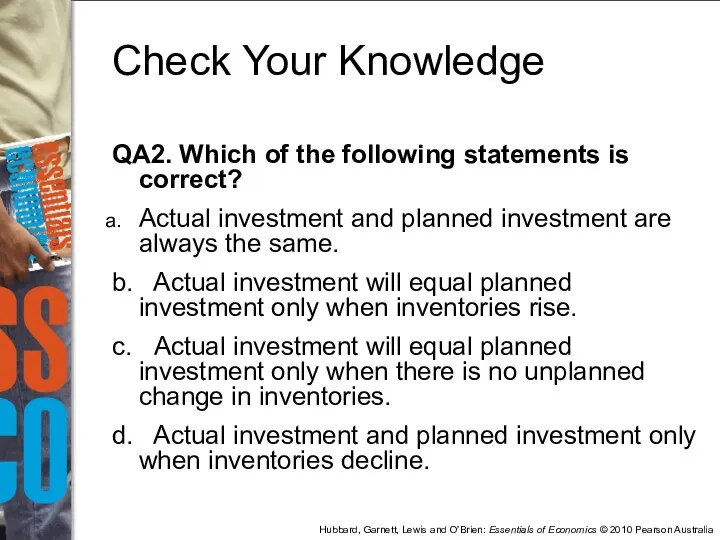
QA2. Which of the following statements is correct?
Actual investment and planned
QA2. Which of the following statements is correct?
Actual investment and planned
 Персонал предприятия и оплата труда
 Политика перестройки в сфере экономики
 Методика экономического анализа, способы обработки информации в экономическом анализе
 Организационно-экономические основы управления недвижимостью
 Сущность и характеристики рыночной экономики. (Лекция 1)
 Фискальная(налоговобюджетная) политика государства. Тема 4
 Ways to strengthen your business in an economic crisis
 Формы общественного хозяйства. Товар и деньги
 Экономика организации. Лекция 1
 Основные этапы развития экономической науки — от возникновения до наших дней
 Markets. Competition
 Североамериканское соглашение о свободной торговле и другие формы реализации международного интеграционного процесса
 История экономического районирования России
 Послание Президента Российской Федерации В.В. Путина Федеральному Собранию на 2018 год
 Специализированные субъекты предпринимательской деятельности
 Рынок факторов производства. Рынок труда
 Провалы рынка. Фиаско государства
 Обзор состояния нефтесервисного рынка РФ
 Развитие экономической мысли в первой половине XX века
 Не? Қашан? Қайда?
 Структура автоматизированной системы промышленного предприятия
 Развитие сектора услуг как фактор и возможность экономического роста РБ
 Разработка модели экономической надежности предприятия. Методы управления рисками на предприятии
 Мировая торговля и международная конкурентоспособность стран. Тема 2.1
 Система ціноутворення
 Общенаучные и специальные методологические подходы и методы проведения экономических исследований
 Муниципальное образование город Обнинск
 Unternehmertum in Belarus