- Forecast combinations

Содержание
- 2. Lecture Objectives Introduce the idea and rationale for forecast averaging Identify forecast averaging implementation issues Become
- 3. Introduction Usually, multiple forecasts are available to decision makers Differences in forecasts reflect: differences in subjective
- 4. Introduction Disadvantages of using a single forecasting model: may contain misspecifications of an unknown form e.g.,
- 5. Outline of the lecture What is a combination of forecasts? The theoretical problem and implementation issues
- 6. Part I. What is a combination of forecasts? General framework and notation The forecast combination problem
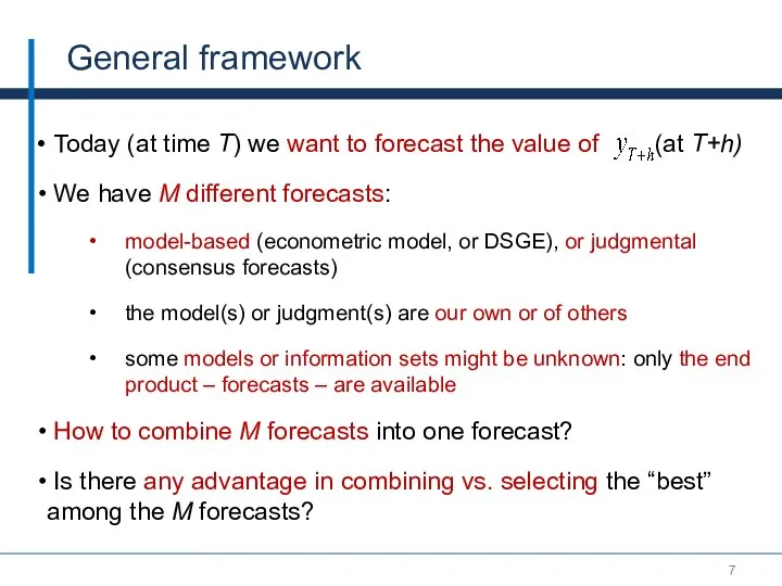
- 7. General framework Today (at time T) we want to forecast the value of (at T+h) We
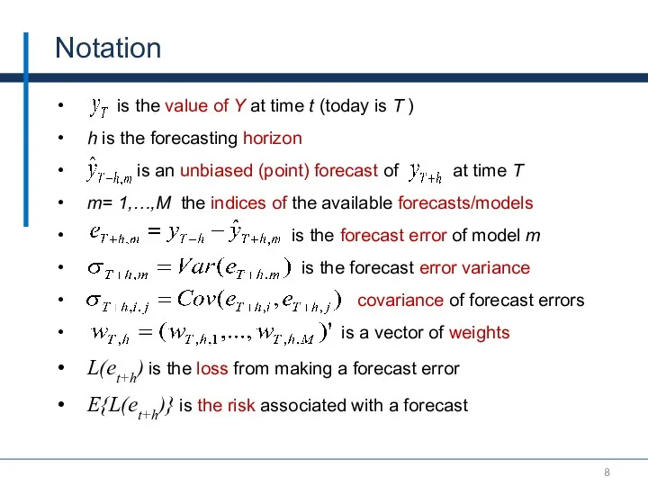
- 8. Notation is the value of Y at time t (today is T ) h is the
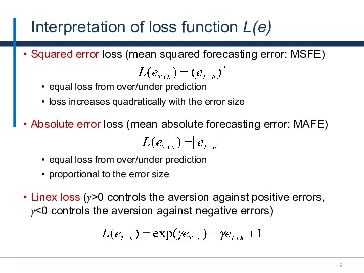
- 9. Interpretation of loss function L(e) Squared error loss (mean squared forecasting error: MSFE) equal loss from
- 10. A combined forecast is a weighted average of M forecasts: The forecast combination problem can be
- 11. Clarification: combining forecasting errors Notice that since then Hence, if weights sum to one, then the
- 12. Summary: what is the problem all about? (II) We want to find optimal weights (the theoretical
- 13. General problem of finding optimal forecast combination Let: u an (M x 1) vector of 1’s,
- 14. Issues and clarifications Do weights have to sum to one? If forecasts are unbiased, this guarantees
- 15. Summary: what is the problem all about? (I) Observations of a variable Y Forecast observations of
- 16. Part II. The theoretical problem and implementation issues A simple example with only 2 forecasts The
- 17. Optimal weights in population (M = 2) Result 1: The solution to Problem 1 is weight
- 18. Interpreting the optimal weights in population Consider the ratio of weights A larger weight is assigned
- 19. Result: Forecast combination reduces error variance Compute the expected MSFE with the optimal weights: |ρ| ≤
- 20. Estimating Σ The key ingredient for finding the optimal weights is the forecast error covariance matrix,
- 21. Issues with estimating Σ Is the estimate of based on the past forecasting errors “good”? If
- 22. Optimality of equal weights The simplest possible averaging scheme uses equal weights The equal weights are
- 23. Part III. Methods to estimate the weights: M is small relative to T (M
- 24. To combine or not to combine? Assess if one forecast encompasses information in other forecasts For
- 25. OLS estimates of the optimal weights Recall the general problem of estimating wm for m forecasts
- 26. Reducing the dependency on sampling errors Assume that estimate is affected by a sampling error (e.g.,
- 27. Part IV. Methods to estimate the weights: when M is large relative to T
- 28. Premise: problems with OLS weights The problem with OLS weights: If M is large relative to
- 29. MSFE weights (or relative performance weights) Relative performance weights An alternative to the of OLS weights:
- 30. Emphasizing recent performance Compute: where is the number of periods with δ(t)>0 and δ(t) can be
- 31. Shrinking relative performance Consider instead As parameter k 0 the relative performance of a particular model
- 32. MSFE weights ignore correlations between forecasting errors Ignoring it, when it is present decreases efficiency –
- 33. Rank-based forecast combination Aiolfi and Timmerman (2006) allow the weights to be inversely related to the
- 34. Trimming In forecast combination, it is often advantageous to discard models with the worst and best
- 35. Example Stock and Watson (2003): relative forecasting performance of various forecast combination schemes versus the AR
- 36. Part V. Improving the Estimates of the Theoretical Model Performance: Knowing the parameters in the model
- 37. Question So far we assumed that we do not know models from which forecasts originate Would
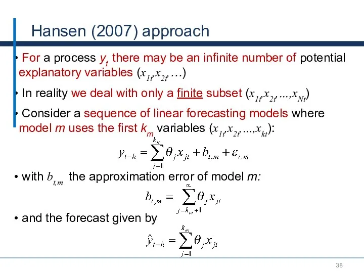
- 38. Hansen (2007) approach For a process yt there may be an infinite number of potential explanatory
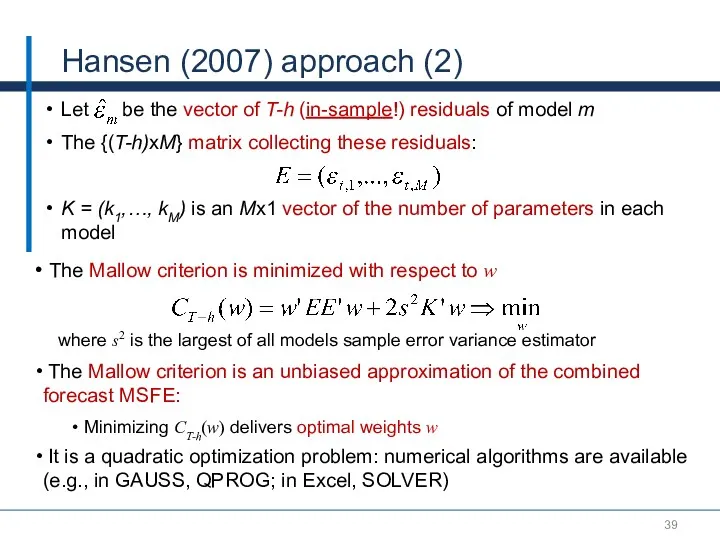
- 39. Hansen (2007) approach (2) Let be the vector of T-h (in-sample!) residuals of model m The
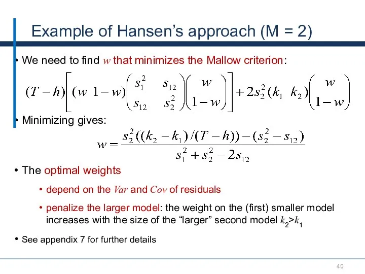
- 40. Example of Hansen’s approach (M = 2) We need to find w that minimizes the Mallow
- 41. Conclusions – Key Takeaways Combined forecasts imply diversification of risk (provided not all the models suffer
- 42. Thank You!
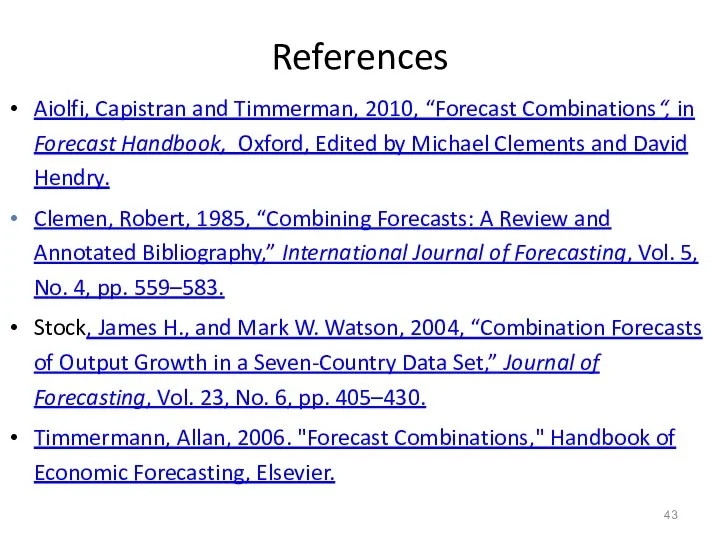
- 43. References Aiolfi, Capistran and Timmerman, 2010, “Forecast Combinations“, in Forecast Handbook, Oxford, Edited by Michael Clements
- 44. Appendix
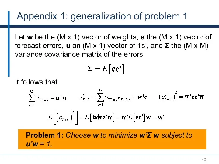
- 45. Appendix 1: generalization of problem 1 Let w be the (M x 1) vector of weights,
- 46. Result 1: Let u be an (M x 1) vector of 1s’ and ΣT,h the variance-covariance
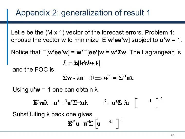
- 47. Appendix 2: generalization of result 1 Let e be the (M x 1) vector of the
- 48. Appendix 2: generalization of result 1 (M = 2) Let Σt,h be the variance-covariance matrix of
- 49. Optimal weights in population (M = 2) Result 1: The solution to Problem 1 is weight
- 50. Appendix 3 Notice that Need to show that the following inequality holds and that Rearrange the
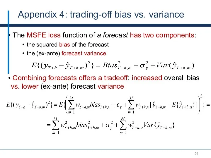
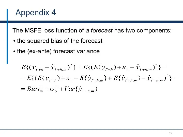
- 51. Appendix 4: trading-off bias vs. variance The MSFE loss function of a forecast has two components:
- 52. Appendix 4 The MSFE loss function of a forecast has two components: the squared bias of
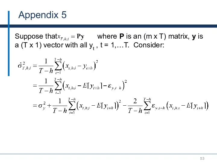
- 53. Appendix 5 Suppose that where P is an (m x T) matrix, y is a (T
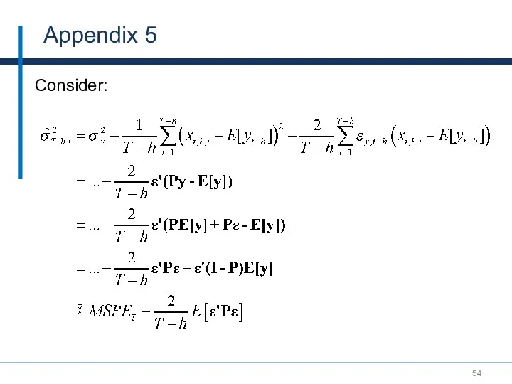
- 54. Appendix 5 Consider:
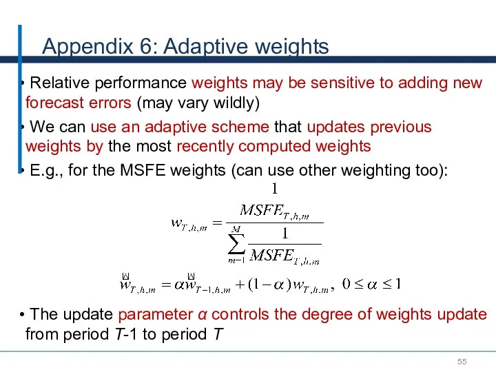
- 55. Appendix 6: Adaptive weights Relative performance weights may be sensitive to adding new forecast errors (may
- 57. Скачать презентацию
Lecture Objectives
Introduce the idea and rationale for forecast averaging
Identify
Lecture Objectives
Introduce the idea and rationale for forecast averaging
Identify
Introduction
Usually, multiple forecasts are available to decision makers
Differences in
Introduction
Usually, multiple forecasts are available to decision makers
Differences in
Introduction
Disadvantages of using a single forecasting model:
may contain misspecifications of
Introduction
Disadvantages of using a single forecasting model:
may contain misspecifications of
Outline of the lecture
What is a combination of forecasts?
The theoretical problem
Outline of the lecture
What is a combination of forecasts?
The theoretical problem
Part I. What is a combination of forecasts?
General framework and notation
The forecast
Part I. What is a combination of forecasts?
General framework and notation
The forecast
General framework
Today (at time T) we want to forecast the
General framework
Today (at time T) we want to forecast the
Notation
is the value of Y at time t (today is
Notation
is the value of Y at time t (today is
Interpretation of loss function L(e)
Squared error loss (mean squared forecasting error:
Interpretation of loss function L(e)
Squared error loss (mean squared forecasting error:
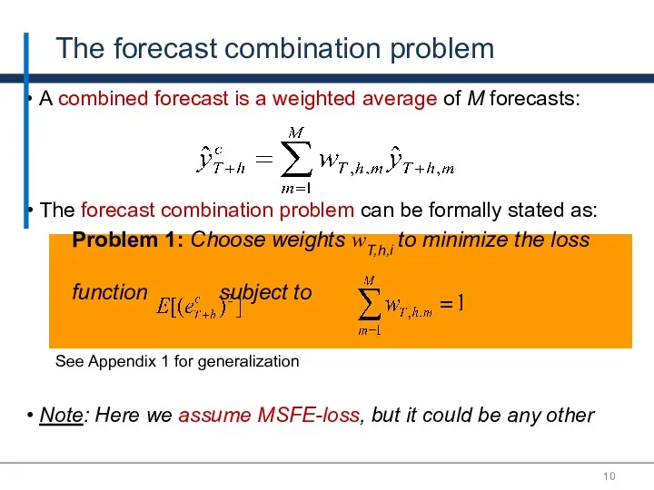
A combined forecast is a weighted average of M forecasts:
The
A combined forecast is a weighted average of M forecasts:
The
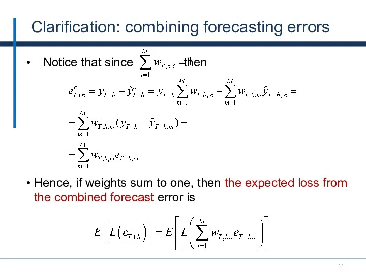
Clarification: combining forecasting errors
Notice that since then
Hence, if weights sum to
Clarification: combining forecasting errors
Notice that since then
Hence, if weights sum to
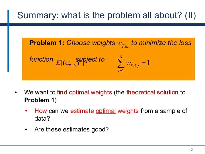
Summary: what is the problem all about? (II)
We want to find
Summary: what is the problem all about? (II)
We want to find
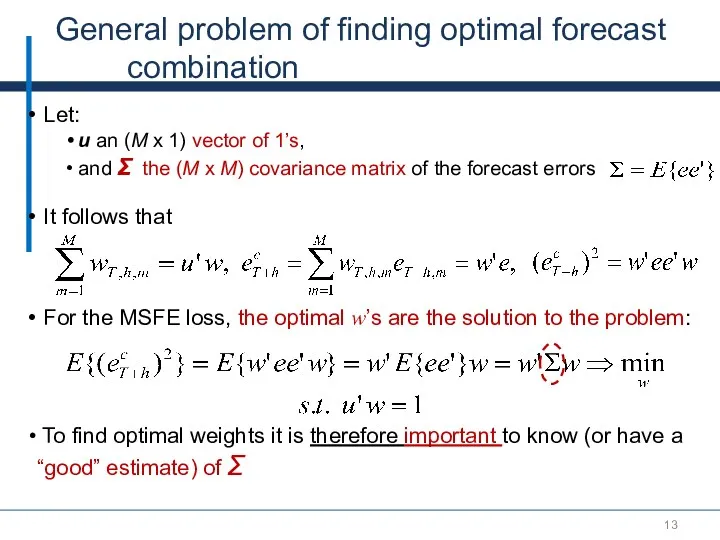
General problem of finding optimal forecast combination
Let:
u an (M
General problem of finding optimal forecast combination
Let:
u an (M
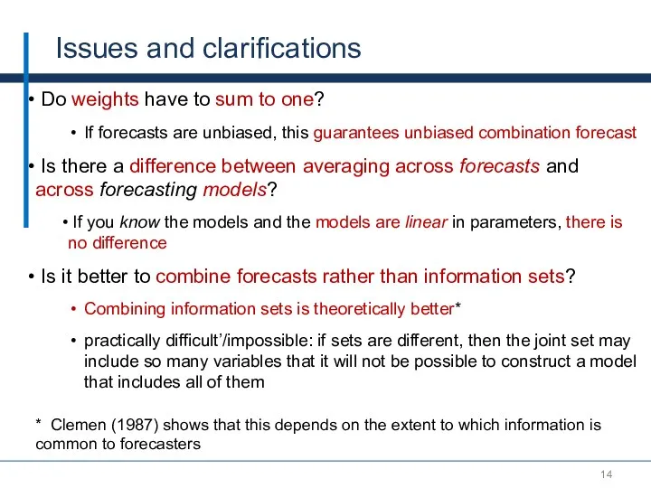
Issues and clarifications
Do weights have to sum to one?
If forecasts
Issues and clarifications
Do weights have to sum to one?
If forecasts
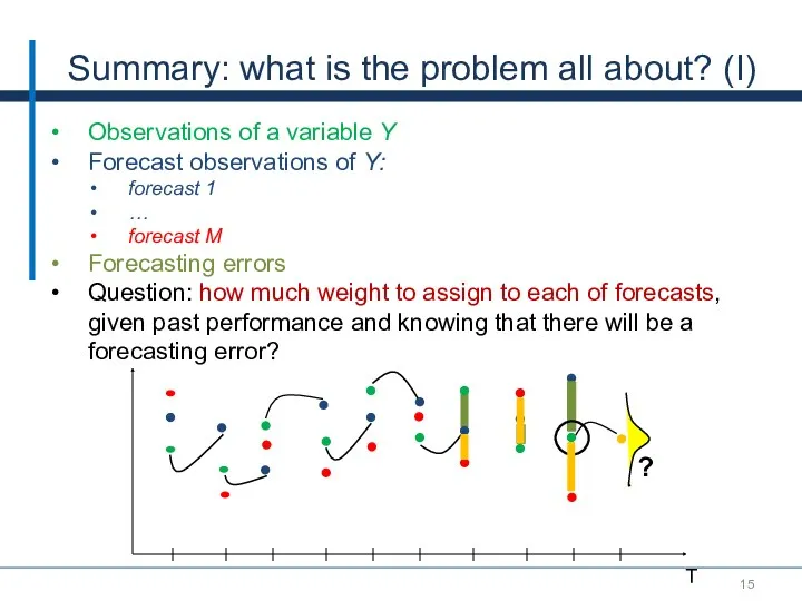
Summary: what is the problem all about? (I)
Observations of a variable
Summary: what is the problem all about? (I)
Observations of a variable
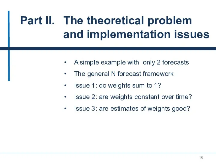
Part II. The theoretical problem and implementation issues
A simple example with only
Part II. The theoretical problem and implementation issues
A simple example with only
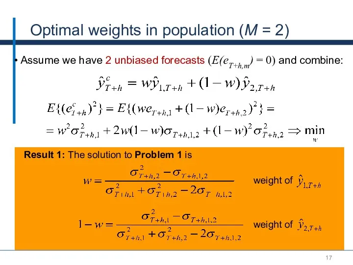
Optimal weights in population (M = 2)
Result 1: The solution to
Optimal weights in population (M = 2)
Result 1: The solution to
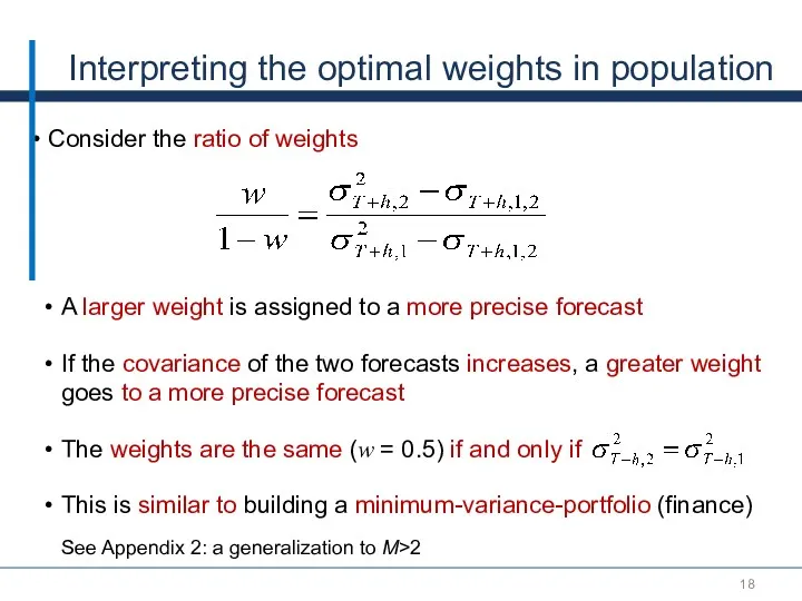
Interpreting the optimal weights in population
Consider the ratio of weights
A
Interpreting the optimal weights in population
Consider the ratio of weights
A
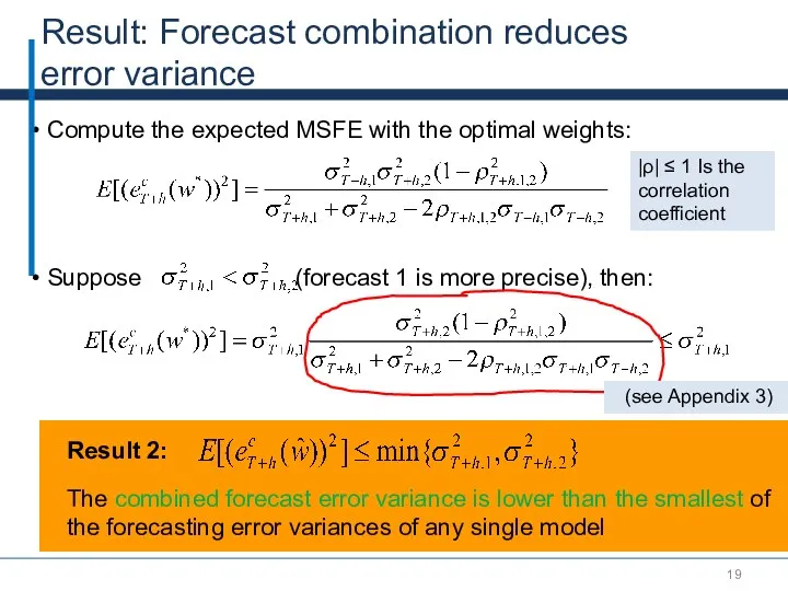
Result: Forecast combination reduces
error variance
Compute the expected MSFE with the
Result: Forecast combination reduces
error variance
Compute the expected MSFE with the
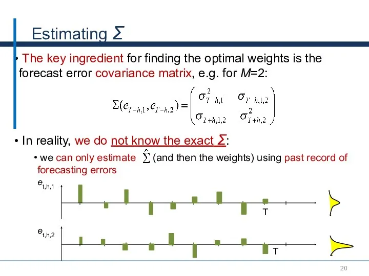
Estimating Σ
The key ingredient for finding the optimal weights is
Estimating Σ
The key ingredient for finding the optimal weights is
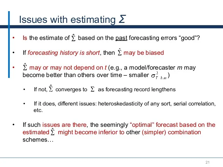
Issues with estimating Σ
Is the estimate of based on the
Issues with estimating Σ
Is the estimate of based on the
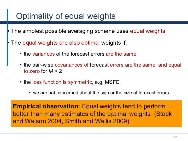
Optimality of equal weights
The simplest possible averaging scheme uses equal
Optimality of equal weights
The simplest possible averaging scheme uses equal
Part III. Methods to estimate the weights:
M is small relative to
Part III. Methods to estimate the weights:
M is small relative to
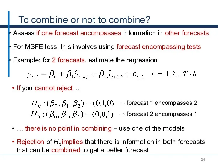
To combine or not to combine?
Assess if one forecast encompasses
To combine or not to combine?
Assess if one forecast encompasses
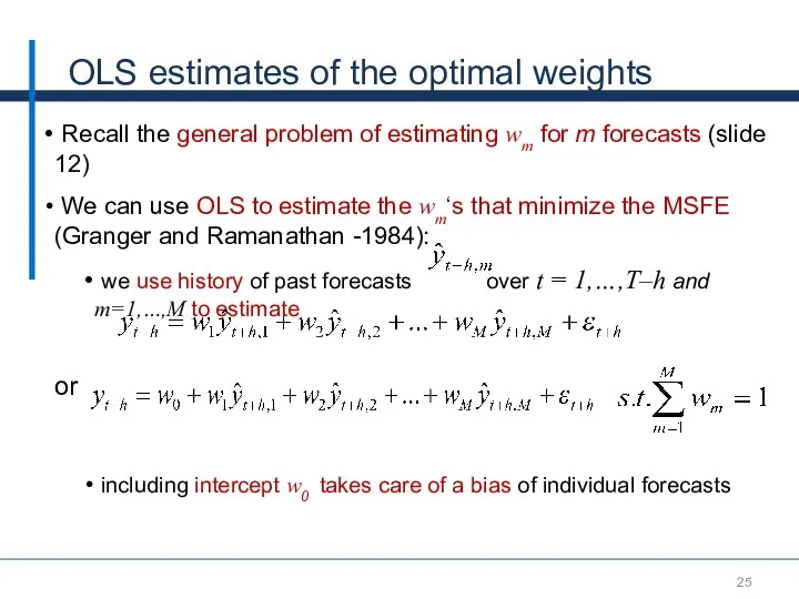
OLS estimates of the optimal weights
Recall the general problem of
OLS estimates of the optimal weights
Recall the general problem of
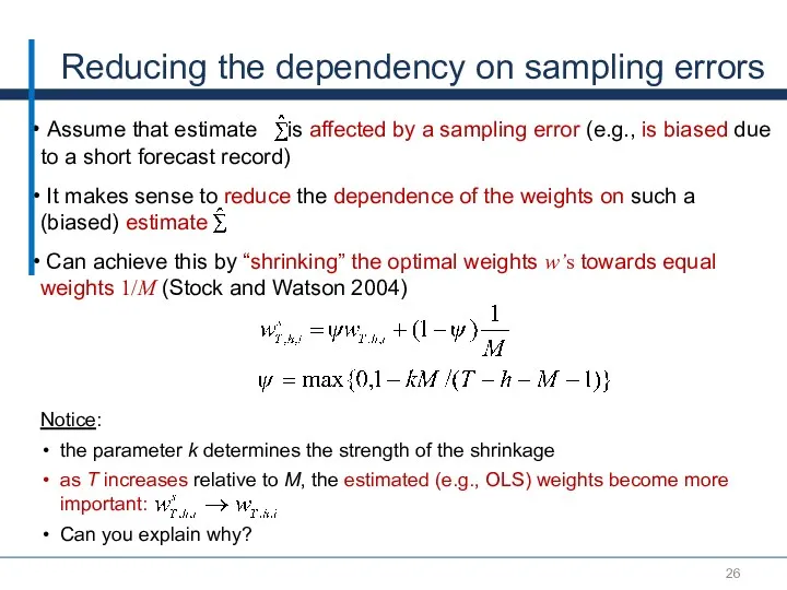
Reducing the dependency on sampling errors
Assume that estimate is affected
Reducing the dependency on sampling errors
Assume that estimate is affected
Part IV. Methods to estimate the weights: when M is large relative
Part IV. Methods to estimate the weights: when M is large relative
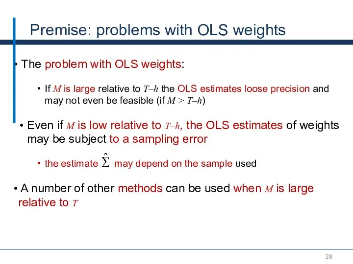
Premise: problems with OLS weights
The problem with OLS weights:
If M
Premise: problems with OLS weights
The problem with OLS weights:
If M
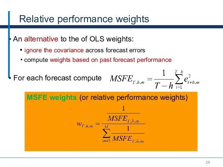
MSFE weights (or relative performance weights)
Relative performance weights
An alternative
MSFE weights (or relative performance weights)
Relative performance weights
An alternative
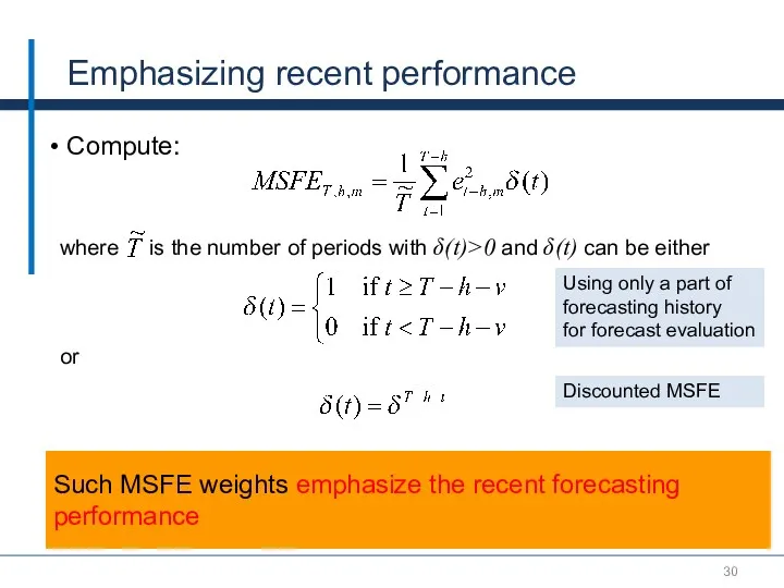
Emphasizing recent performance
Compute:
where is the number of periods with δ(t)>0
Emphasizing recent performance
Compute:
where is the number of periods with δ(t)>0
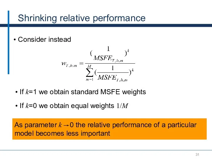
Shrinking relative performance
Consider instead
As parameter k 0 the relative performance
Shrinking relative performance
Consider instead
As parameter k 0 the relative performance
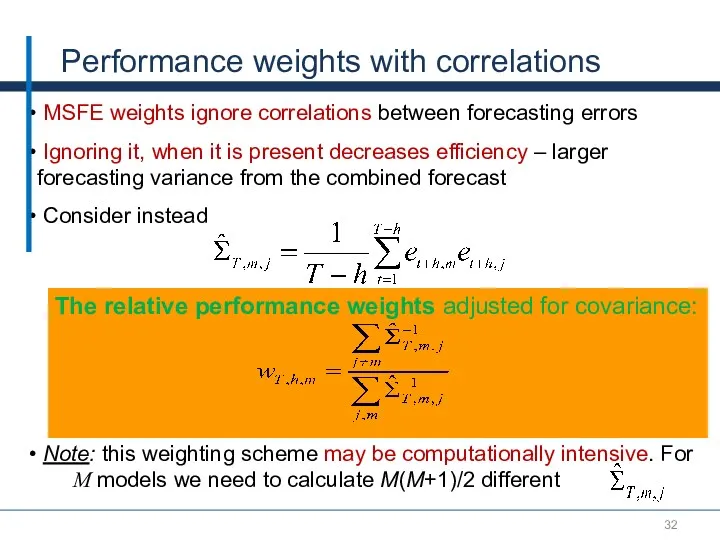
MSFE weights ignore correlations between forecasting errors
Ignoring it, when
MSFE weights ignore correlations between forecasting errors
Ignoring it, when
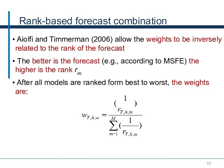
Rank-based forecast combination
Aiolfi and Timmerman (2006) allow the weights to
Rank-based forecast combination
Aiolfi and Timmerman (2006) allow the weights to
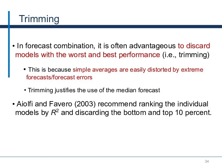
Trimming
In forecast combination, it is often advantageous to discard models
Trimming
In forecast combination, it is often advantageous to discard models
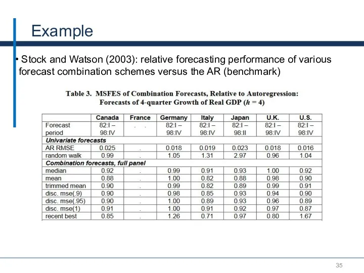
Example
Stock and Watson (2003): relative forecasting performance of various forecast
Example
Stock and Watson (2003): relative forecasting performance of various forecast
Part V. Improving the Estimates of the Theoretical Model Performance: Knowing the
Part V. Improving the Estimates of the Theoretical Model Performance: Knowing the
Question
So far we assumed that we do not know models
Question
So far we assumed that we do not know models
Hansen (2007) approach
For a process yt there may be an
Hansen (2007) approach
For a process yt there may be an
Hansen (2007) approach (2)
Let be the vector of T-h (in-sample!) residuals
Hansen (2007) approach (2)
Let be the vector of T-h (in-sample!) residuals
Example of Hansen’s approach (M = 2)
We need to find
Example of Hansen’s approach (M = 2)
We need to find
Conclusions – Key Takeaways
Combined forecasts imply diversification of risk (provided not
Conclusions – Key Takeaways
Combined forecasts imply diversification of risk (provided not

Thank You!
Thank You!
References
Aiolfi, Capistran and Timmerman, 2010, “Forecast Combinations“, in Forecast Handbook, Oxford,
References
Aiolfi, Capistran and Timmerman, 2010, “Forecast Combinations“, in Forecast Handbook, Oxford,

Appendix
Appendix
Appendix 1: generalization of problem 1
Let w be the (M x
Appendix 1: generalization of problem 1
Let w be the (M x
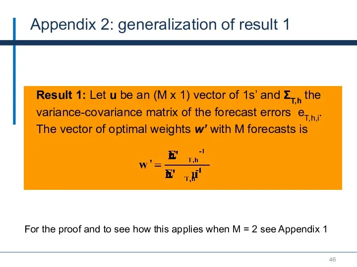
Result 1: Let u be an (M x 1) vector of
Result 1: Let u be an (M x 1) vector of
Appendix 2: generalization of result 1
Let e be the (M x
Appendix 2: generalization of result 1
Let e be the (M x
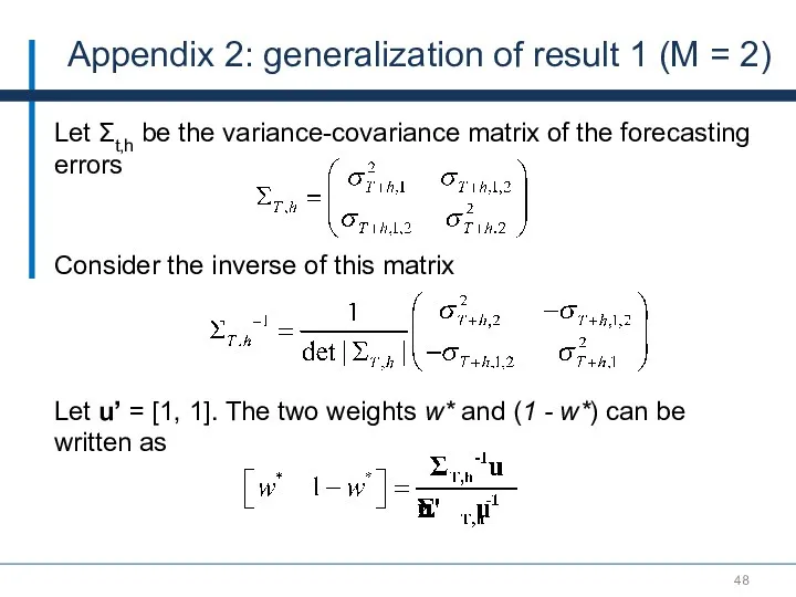
Appendix 2: generalization of result 1 (M = 2)
Let Σt,h be
Appendix 2: generalization of result 1 (M = 2)
Let Σt,h be
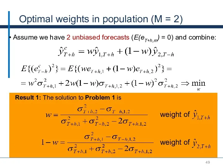
Optimal weights in population (M = 2)
Result 1: The solution to
Optimal weights in population (M = 2)
Result 1: The solution to
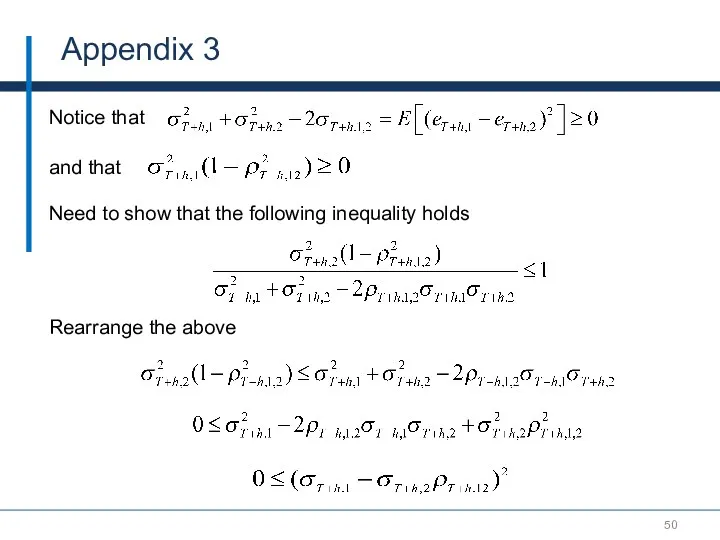
Appendix 3
Notice that
Need to show that the following inequality holds
and that
Rearrange
Appendix 3
Notice that
Need to show that the following inequality holds
and that
Rearrange
Appendix 4: trading-off bias vs. variance
The MSFE loss function of
Appendix 4: trading-off bias vs. variance
The MSFE loss function of
Appendix 4
The MSFE loss function of a forecast has two components:
the
Appendix 4
The MSFE loss function of a forecast has two components:
the
Appendix 5
Suppose that where P is an (m x T) matrix,
Appendix 5
Suppose that where P is an (m x T) matrix,
Appendix 5
Consider:
Appendix 5
Consider:
Appendix 6: Adaptive weights
Relative performance weights may be sensitive to
Appendix 6: Adaptive weights
Relative performance weights may be sensitive to
 Таур қорын,қаржыны және басқа да активтерді нормалау. Тауардың босатылу көлемін қамтамасыз ету
 Економічний розвиток України в умовах радянської економічної системи та його трактування в економічній думці
 Курс Экономика. Лекция 2. Базовые экономические понятия
 Аштық көрсеткішінің индексі
 АСЕАН - история создания, цели, задачи, членство, результаты деятельности
 Экономика. Вопросы 1-2-3 темы
 Факторы, определяющие спрос на труд, и предложения труда
 Поведение фирмы
 Товар и его свойства
 Эластичность спроса и предложения. Рыночное равновесие
 Сущность управления затратами предприятия
 Сегодняшние проблемы российской экономики
 Макроэкономическая нестабильность
 Глобальные проблемы современности
 Развитие кредитования юридических лиц
 Метод проектов на уроках экономики
 Туризм-экономика саласы ретінде
 Прогнозы развития российской экономики на 2016-2018 годы
 Спрос, предложение и рыночное равновесие
 Организация работ по ТО и ТР автомобилей KIA RIO с детальной разработкой зоны участка УМР на примере ООО Нормандия - Авто
 Ценообразование
 Планирования производства на сельскохозяйственных предприятиях. (Тема 3)
 Мемлекет басшысы Н.Назарбаевтың Қазақстан халқына Жолдауы. 2015 жылғы 30 қараша
 Муниципальное образование Чаинский район
 Ограниченность – основная проблема экономики
 Типы экономических систем
 Статистика уровня жизни населения
 Совершенная и несовершенная конкуренция. Тема 7