- Growth theory: the economy in the very long run

Содержание
- 2. ECONOMIC GROWTH I: CAPITAL ACCUMULATION & POPULATION GROWTH 8
- 3. 8-1 The Accumulation of Capital 8-2 The Golden Rule Level of Capital 8-3 Population Growth
- 4. The Solow growth model shows how saving, population growth, technological progress Level & Growth of output
- 5. Income and poverty in the world selected countries, 2010 Indonesia Uruguay Poland Senegal Kyrgyz Republic Nigeria
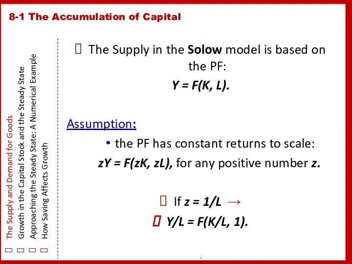
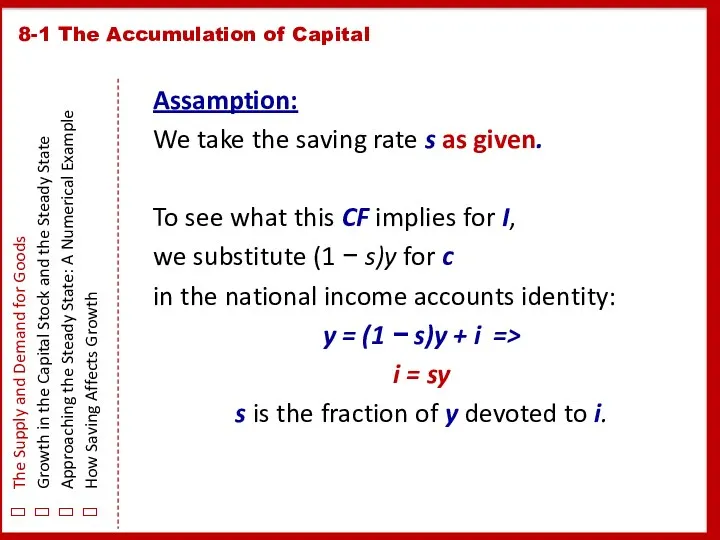
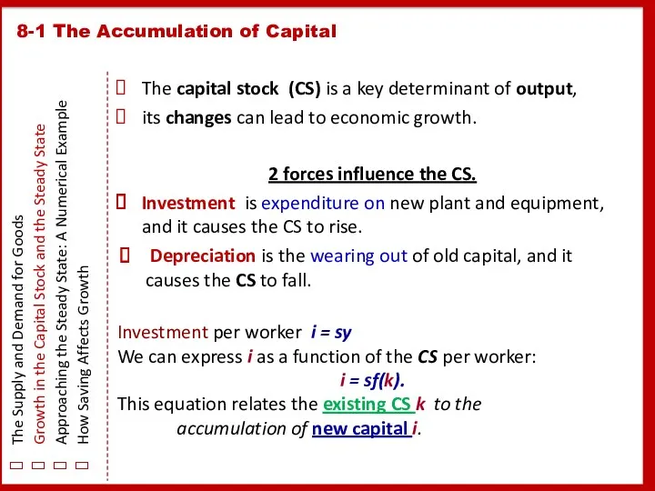
- 6. 8-1 The Accumulation of Capital The Supply and Demand for Goods Growth in the Capital Stock
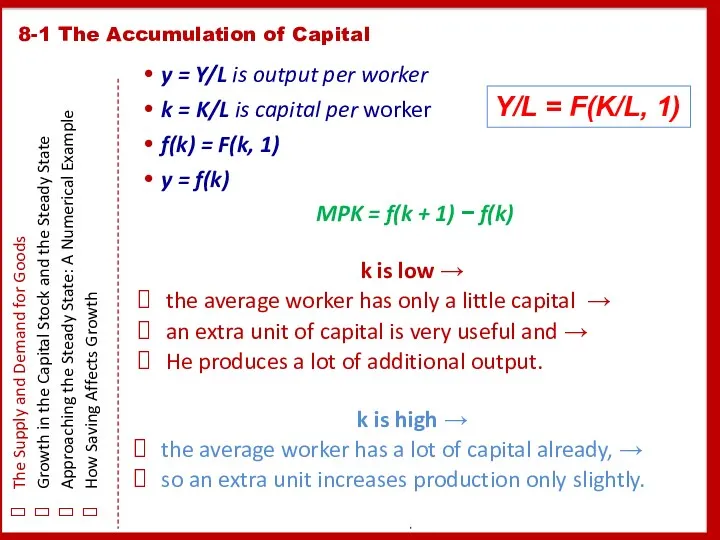
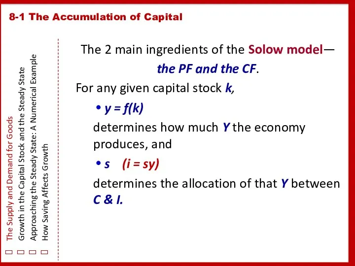
- 7. y = Y/L is output per worker k = K/L is capital per worker f(k) =
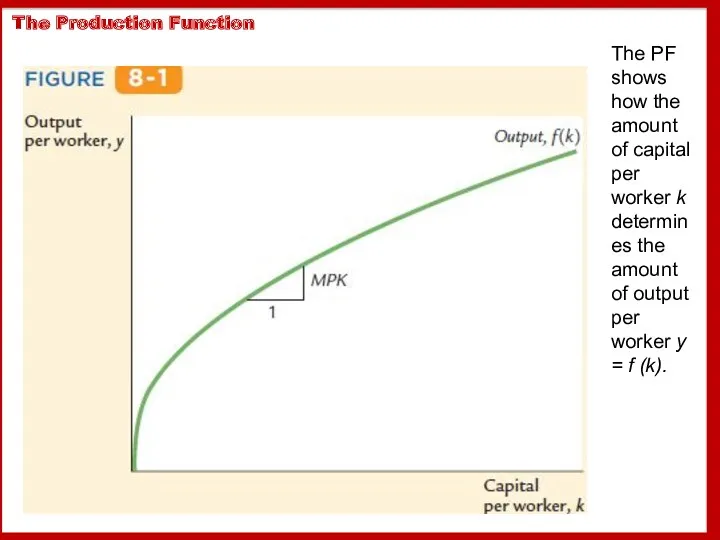
- 8. The Production Function The PF shows how the amount of capital per worker k determines the
- 9. 8-1 The Accumulation of Capital The Supply and Demand for Goods Growth in the Capital Stock
- 10. 8-1 The Accumulation of Capital The Supply and Demand for Goods Growth in the Capital Stock
- 11. 8-1 The Accumulation of Capital The Supply and Demand for Goods Growth in the Capital Stock
- 12. 8-1 The Accumulation of Capital The Supply and Demand for Goods Growth in the Capital Stock
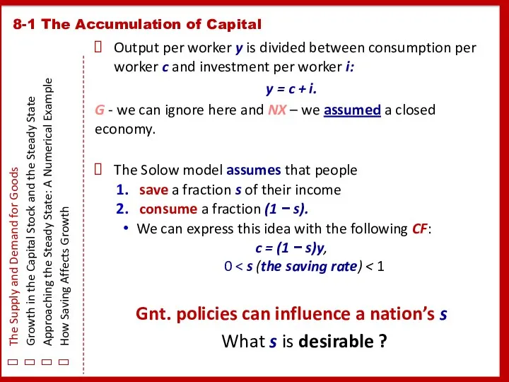
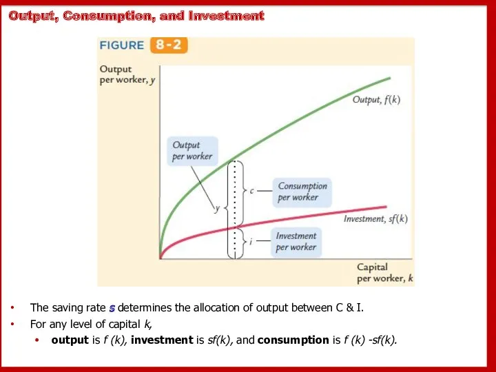
- 13. Output, Consumption, and Investment The saving rate s determines the allocation of output between C &
- 14. Depreciation is a constant fraction of the CS wears out every year. Depreciation is therefore proportional
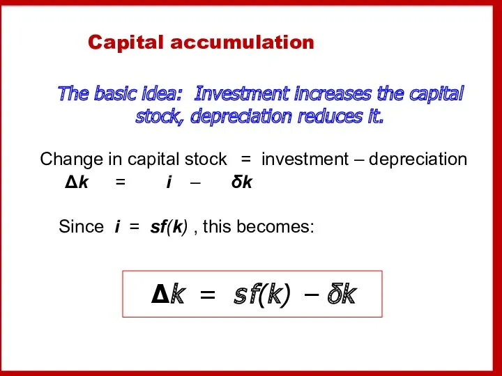
- 15. Capital accumulation Change in capital stock = investment – depreciation Δk = i – δk Since
- 16. The equation of motion for k The Solow model’s central equation Determines behavior of capital over
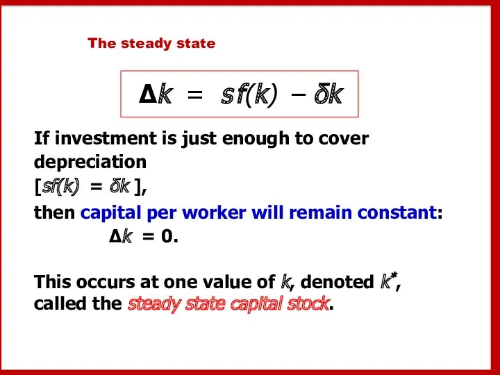
- 17. The steady state If investment is just enough to cover depreciation [sf(k) = δk ], then
- 18. The steady state
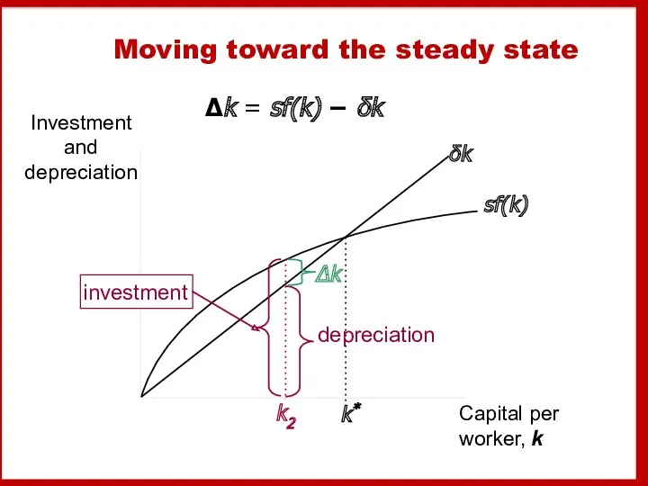
- 19. Moving toward the steady state Δk = sf(k) − δk
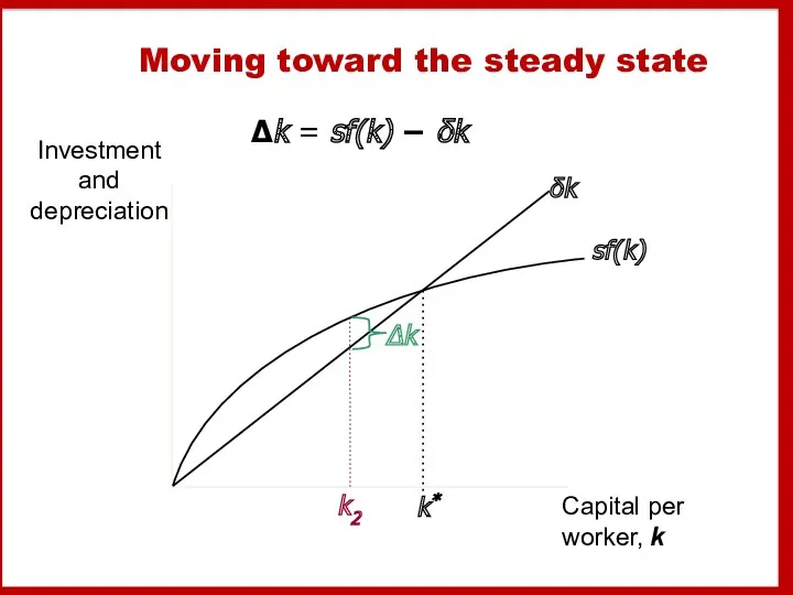
- 20. Moving toward the steady state Δk = sf(k) − δk
- 21. Moving toward the steady state Δk = sf(k) − δk k2
- 22. Moving toward the steady state Δk = sf(k) − δk k2
- 23. Moving toward the steady state Δk = sf(k) − δk
- 24. Moving toward the steady state Δk = sf(k) − δk k2 k3
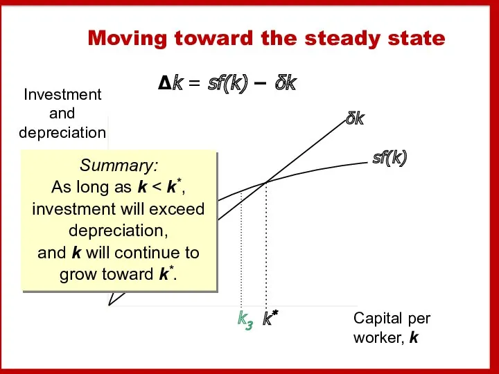
- 25. Moving toward the steady state Δk = sf(k) − δk k3 Summary: As long as k
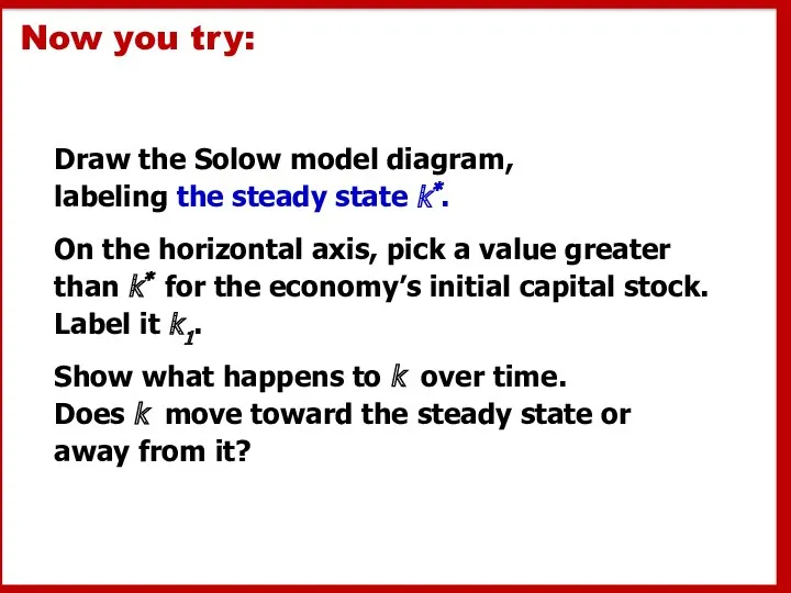
- 26. Now you try: Draw the Solow model diagram, labeling the steady state k*. On the horizontal
- 27. A numerical example Production function (aggregate): To derive the per-worker production function, divide through by L:
- 28. A numerical example, cont. Assume: s = 0.3 δ= 0.1 initial value of k = 4.0
- 29. Approaching the steady state: A numerical example Year k y c i k k 1 4.000
- 30. Exercise: Solve for the steady state Continue to assume s = 0.3, δ = 0.1, and
- 31. Solution to exercise:
- 32. An increase in the saving rate An increase in the saving rate raises investment… …causing k
- 33. Prediction: Higher s ⇒ higher k*. And since y = f(k) , higher k* ⇒ higher
- 34. International evidence on investment rates and income per person 100 1,000 10,000 100,000 0 5 10
- 35. The Golden Rule: Introduction Different values of s lead to different steady states. How do we
- 36. The Golden Rule capital stock the Golden Rule level of capital, the steady state value of
- 37. Then, graph f(k*) and δk*, look for the point where the gap between them is biggest.
- 38. The Golden Rule capital stock c* = f(k*) − δk* is biggest where the slope of
- 39. The transition to the Golden Rule steady state The economy does NOT have a tendency to
- 40. Starting with too much capital then increasing c* requires a fall in s. In the transition
- 41. Starting with too little capital then increasing c* requires an increase in s. Future generations enjoy
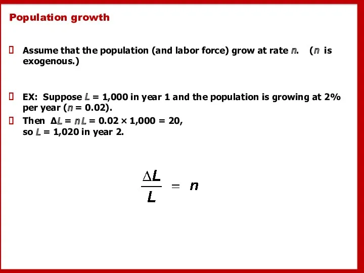
- 42. Population growth Assume that the population (and labor force) grow at rate n. (n is exogenous.)
- 43. Break-even investment (δ + n)k = break-even investment, the amount of investment necessary to keep k
- 44. The equation of motion for k With population growth, the equation of motion for k is
- 45. The Solow model diagram Δk = s f(k) − (δ +n)k
- 46. The impact of population growth Investment, break-even investment Capital per worker, k (δ +n1) k k1*
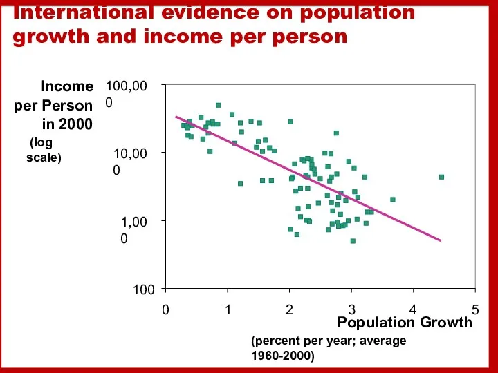
- 47. Prediction: Higher n ⇒ lower k*. And since y = f(k) , lower k* ⇒ lower
- 48. International evidence on population growth and income per person 100 1,000 10,000 100,000 0 1 2
- 49. The Golden Rule with population growth To find the Golden Rule capital stock, express c* in
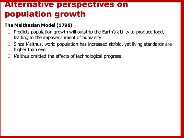
- 50. Alternative perspectives on population growth The Malthusian Model (1798) Predicts population growth will outstrip the Earth’s
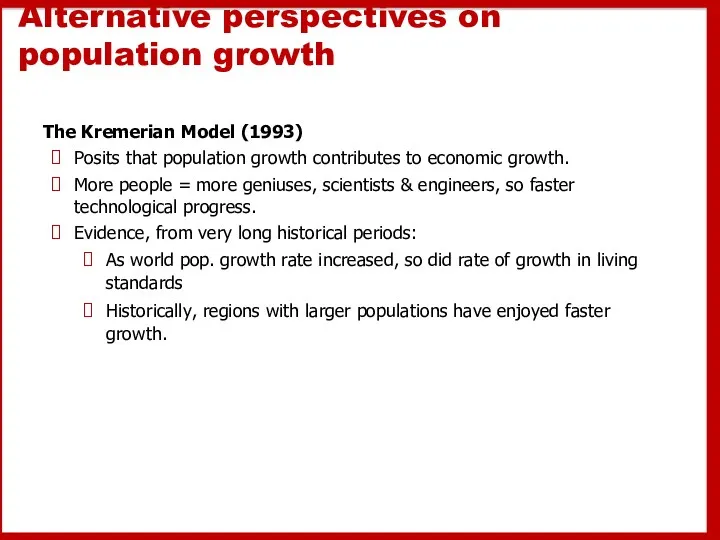
- 51. Alternative perspectives on population growth The Kremerian Model (1993) Posits that population growth contributes to economic
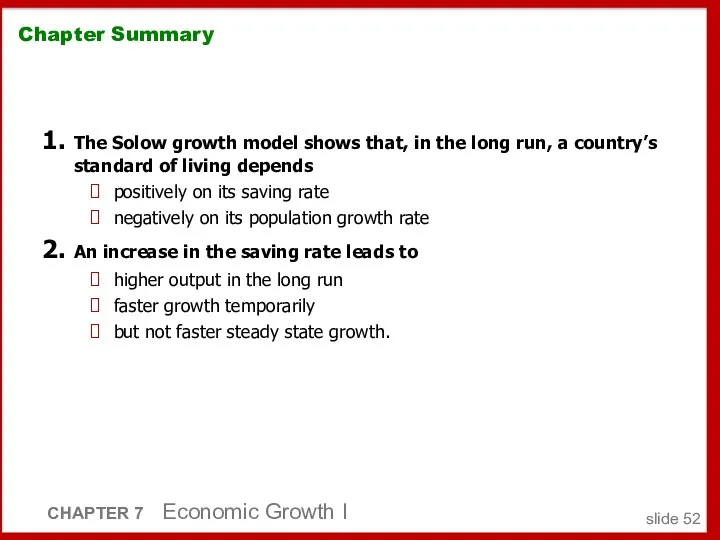
- 52. Chapter Summary 1. The Solow growth model shows that, in the long run, a country’s standard
- 54. Скачать презентацию
ECONOMIC GROWTH I:
CAPITAL ACCUMULATION
&
POPULATION GROWTH
8
ECONOMIC GROWTH I:
CAPITAL ACCUMULATION
&
POPULATION GROWTH
8
8-1 The Accumulation of Capital
8-2 The Golden Rule Level of
8-1 The Accumulation of Capital
8-2 The Golden Rule Level of
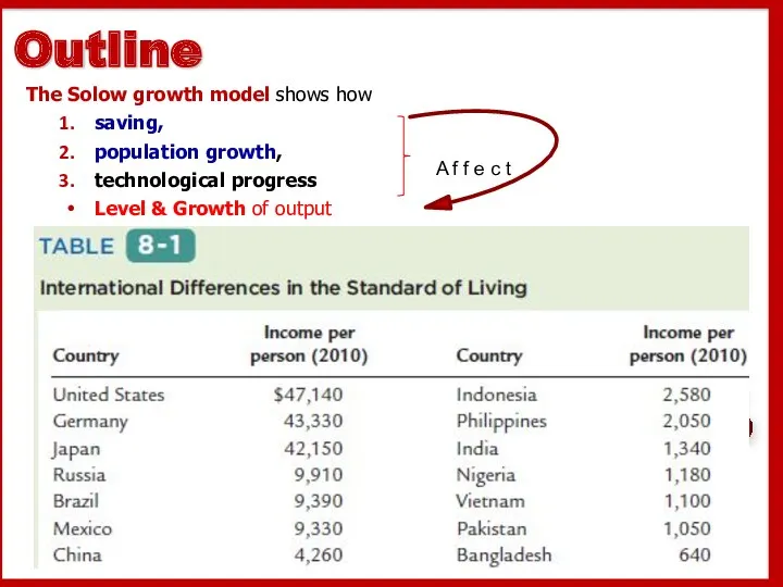
The Solow growth model shows how
saving,
population growth,
technological progress
The Solow growth model shows how
saving,
population growth,
technological progress
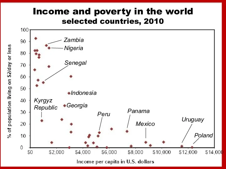
Income and poverty in the world
selected countries, 2010
Indonesia
Uruguay
Poland
Senegal
Kyrgyz Republic
Nigeria
Zambia
Panama
Mexico
Georgia
Peru
Income and poverty in the world
selected countries, 2010
Indonesia
Uruguay
Poland
Senegal
Kyrgyz Republic
Nigeria
Zambia
Panama
Mexico
Georgia
Peru
8-1 The Accumulation of Capital
The Supply and Demand for Goods
Growth in
8-1 The Accumulation of Capital
The Supply and Demand for Goods
Growth in
y = Y/L is output per worker
k = K/L is
y = Y/L is output per worker
k = K/L is
The Production Function
The PF shows how the amount of capital per
The Production Function
The PF shows how the amount of capital per
8-1 The Accumulation of Capital
The Supply and Demand for Goods
Growth in
8-1 The Accumulation of Capital
The Supply and Demand for Goods
Growth in
8-1 The Accumulation of Capital
The Supply and Demand for Goods
Growth in
8-1 The Accumulation of Capital
The Supply and Demand for Goods
Growth in
8-1 The Accumulation of Capital
The Supply and Demand for Goods
Growth in
8-1 The Accumulation of Capital
The Supply and Demand for Goods
Growth in
8-1 The Accumulation of Capital
The Supply and Demand for Goods
Growth in
8-1 The Accumulation of Capital
The Supply and Demand for Goods
Growth in
Output, Consumption, and Investment
The saving rate s determines the allocation of
Output, Consumption, and Investment
The saving rate s determines the allocation of
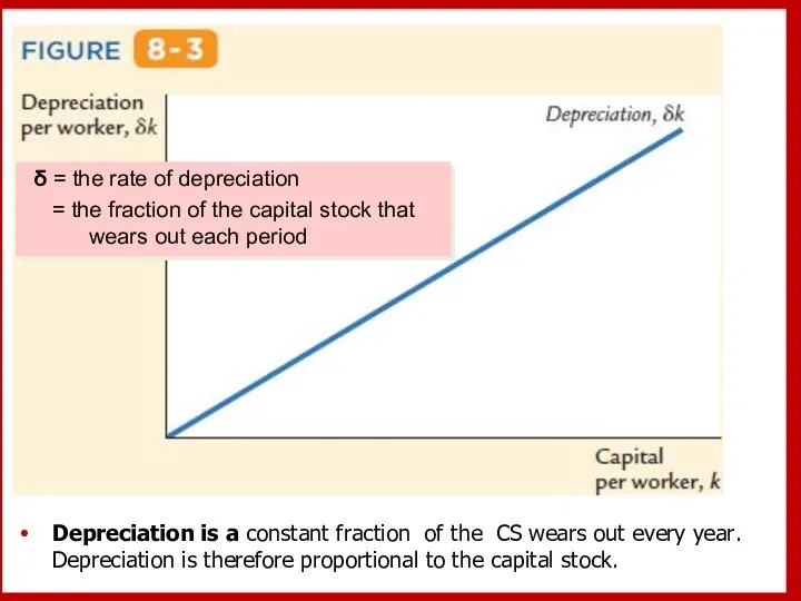
Depreciation is a constant fraction of the CS wears out every
Depreciation is a constant fraction of the CS wears out every
Capital accumulation
Change in capital stock = investment – depreciation
Δk = i –
Capital accumulation
Change in capital stock = investment – depreciation
Δk = i –
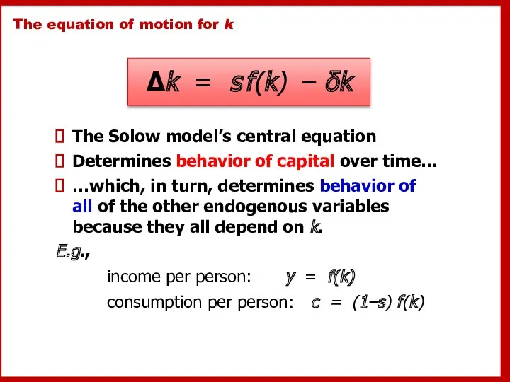
The equation of motion for k
The Solow model’s central equation
Determines behavior
The equation of motion for k
The Solow model’s central equation
Determines behavior
The steady state
If investment is just enough to cover depreciation
[sf(k)
The steady state
If investment is just enough to cover depreciation [sf(k)
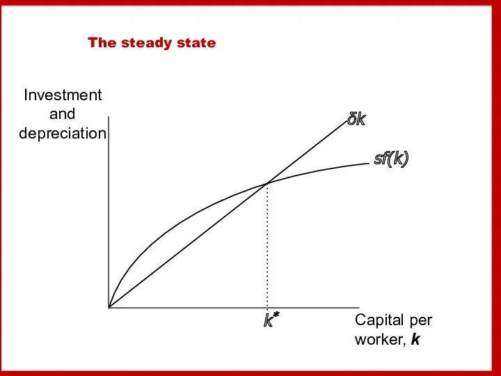
The steady state
The steady state
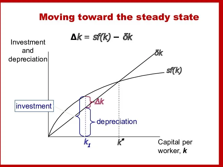
Moving toward the steady state
Δk = sf(k) − δk
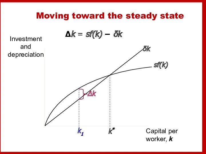
Moving toward the steady state
Δk = sf(k) − δk
Moving toward the steady state
Δk = sf(k) − δk
Moving toward the steady state
Δk = sf(k) − δk
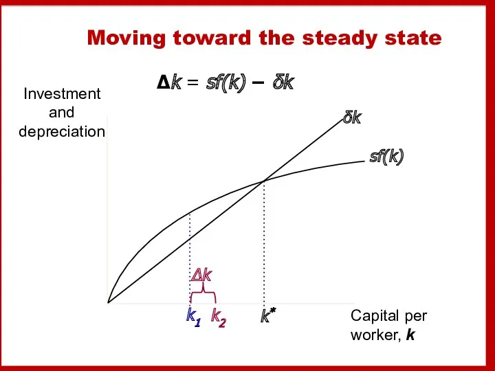
Moving toward the steady state
Δk = sf(k) − δk
k2
Moving toward the steady state
Δk = sf(k) − δk
k2
Moving toward the steady state
Δk = sf(k) − δk
k2
Moving toward the steady state
Δk = sf(k) − δk
k2
Moving toward the steady state
Δk = sf(k) − δk
Moving toward the steady state
Δk = sf(k) − δk

Moving toward the steady state
Δk = sf(k) − δk
k2
k3
Moving toward the steady state
Δk = sf(k) − δk
k2
k3
Moving toward the steady state
Δk = sf(k) − δk
k3
Summary:
As long as
Moving toward the steady state
Δk = sf(k) − δk
k3
Summary: As long as
Now you try:
Draw the Solow model diagram,
labeling the steady state
Now you try:
Draw the Solow model diagram, labeling the steady state
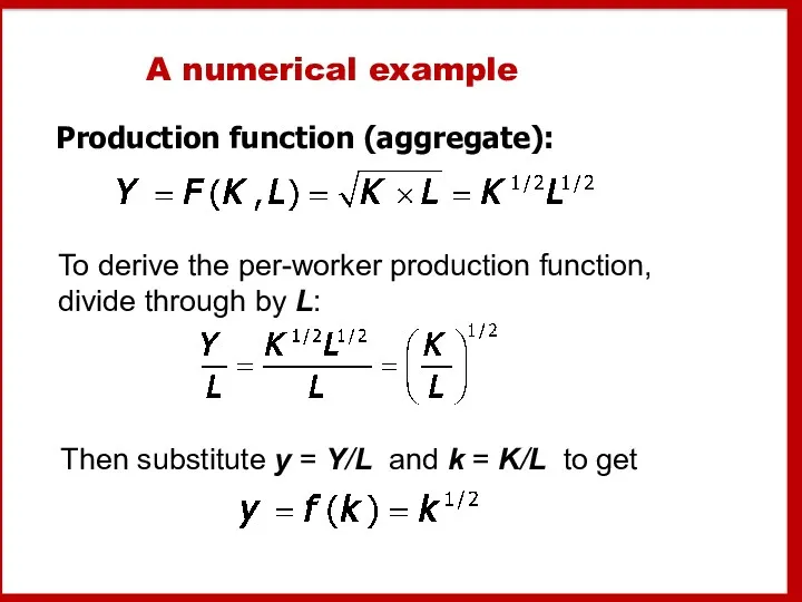
A numerical example
Production function (aggregate):
To derive the per-worker production function, divide
A numerical example
Production function (aggregate):
To derive the per-worker production function, divide
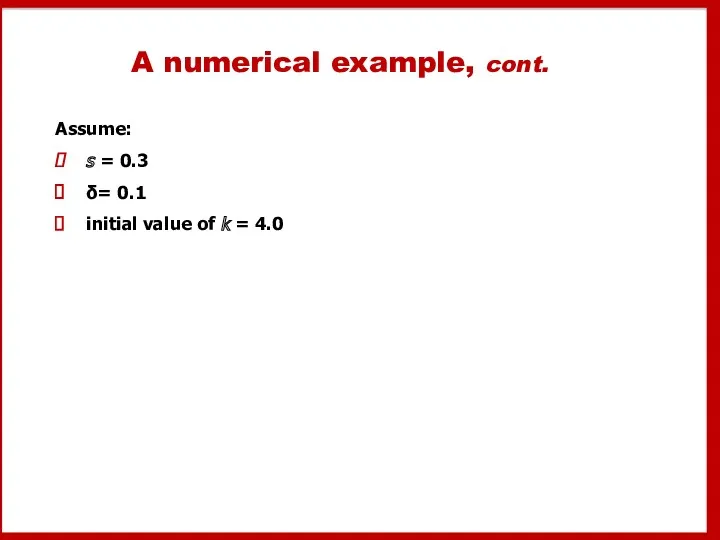
A numerical example, cont.
Assume:
s = 0.3
δ= 0.1
initial value of k =
A numerical example, cont.
Assume:
s = 0.3
δ= 0.1
initial value of k =
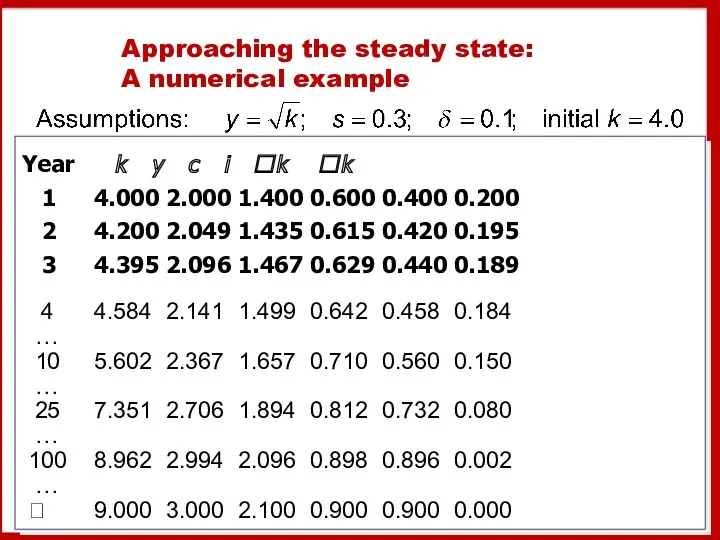
Approaching the steady state:
A numerical example
Year k y c i
Approaching the steady state:
A numerical example
Year k y c i
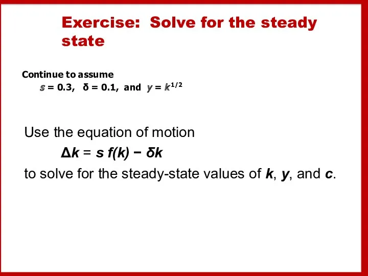
Exercise: Solve for the steady state
Continue to assume
s = 0.3,
Exercise: Solve for the steady state
Continue to assume s = 0.3,
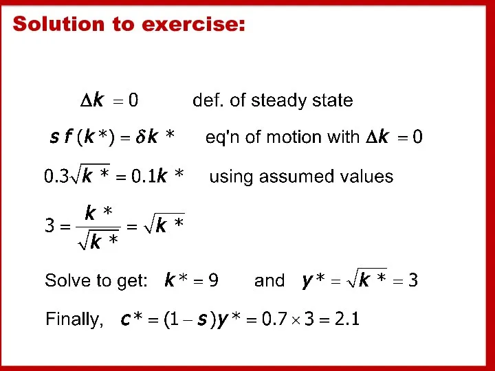
Solution to exercise:
Solution to exercise:
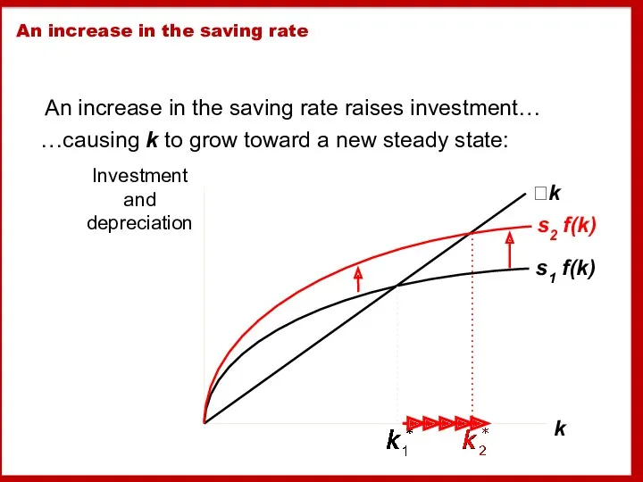
An increase in the saving rate
An increase in the saving rate
An increase in the saving rate
An increase in the saving rate
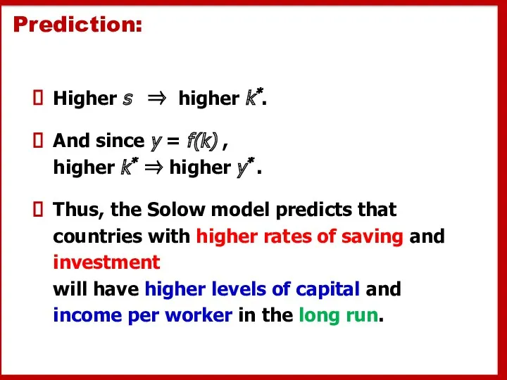
Prediction:
Higher s ⇒ higher k*.
And since y = f(k) ,
Prediction:
Higher s ⇒ higher k*.
And since y = f(k) ,
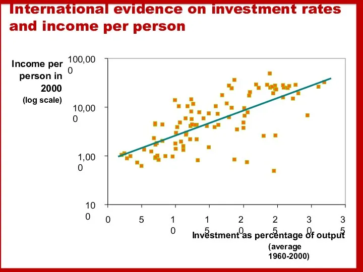
International evidence on investment rates and income per person
100
1,000
10,000
100,000
0
5
10
15
20
25
30
35
Investment as percentage
International evidence on investment rates and income per person
100
1,000
10,000
100,000
0
5
10
15
20
25
30
35
Investment as percentage
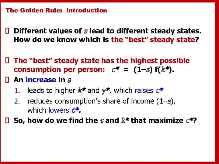
The Golden Rule: Introduction
Different values of s lead to different steady
The Golden Rule: Introduction
Different values of s lead to different steady
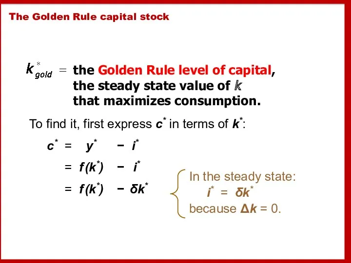
The Golden Rule capital stock
the Golden Rule level of capital,
the
The Golden Rule capital stock
the Golden Rule level of capital, the
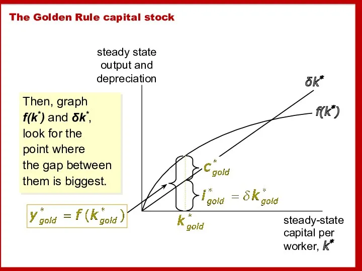
Then, graph
f(k*) and δk*,
look for the
point where
the
Then, graph f(k*) and δk*, look for the point where the
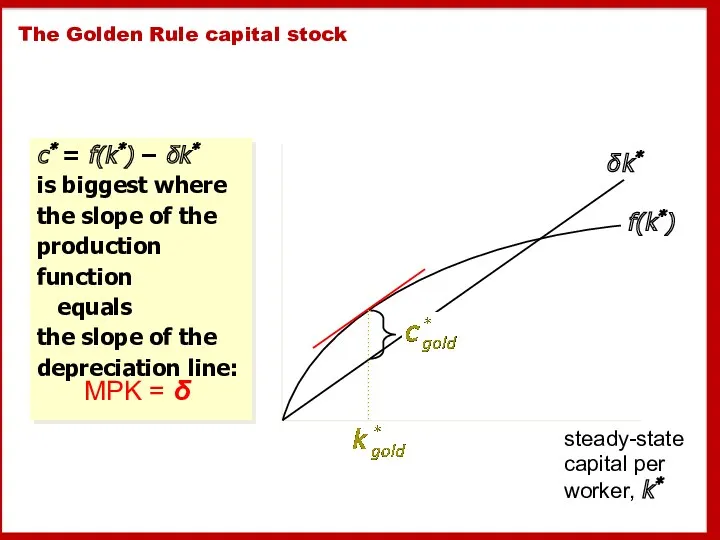
The Golden Rule capital stock
c* = f(k*) − δk*
is biggest where
The Golden Rule capital stock
c* = f(k*) − δk* is biggest where

The transition to the
Golden Rule steady state
The economy does NOT
The transition to the
Golden Rule steady state
The economy does NOT
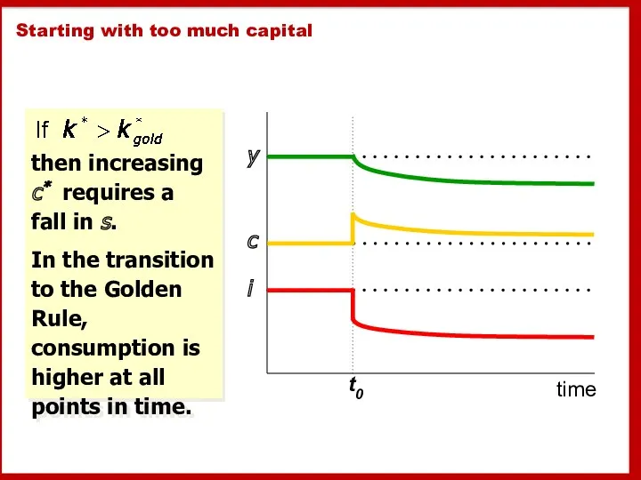
Starting with too much capital
then increasing c* requires a fall in
Starting with too much capital
then increasing c* requires a fall in
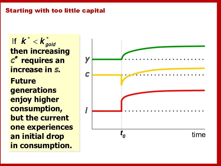
Starting with too little capital
then increasing c* requires an
increase in
Starting with too little capital
then increasing c* requires an
increase in
Population growth
Assume that the population (and labor force) grow at rate
Population growth
Assume that the population (and labor force) grow at rate
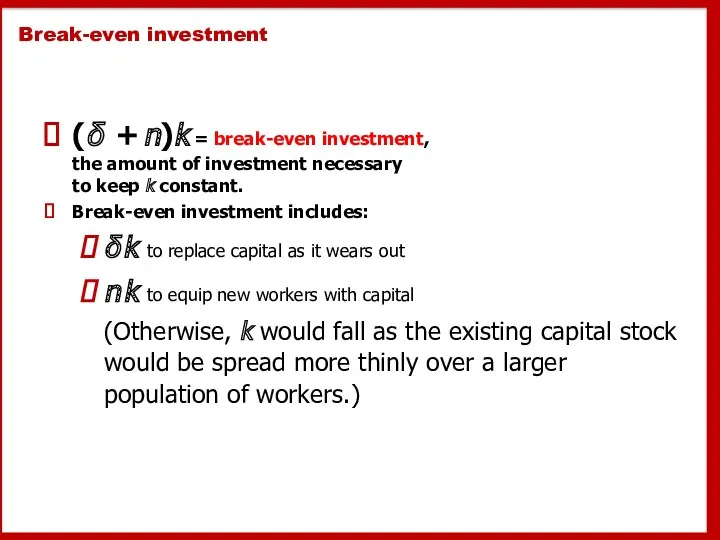
Break-even investment
(δ + n)k = break-even investment,
the amount of investment
Break-even investment
(δ + n)k = break-even investment, the amount of investment
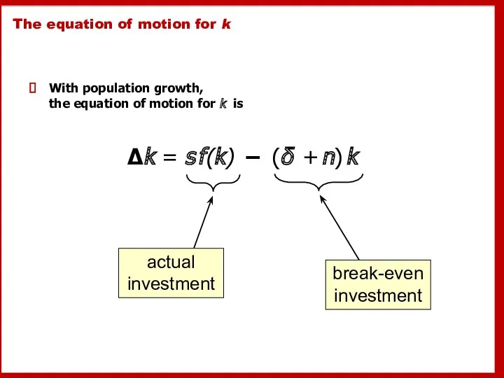
The equation of motion for k
With population growth,
the equation of
The equation of motion for k
With population growth, the equation of
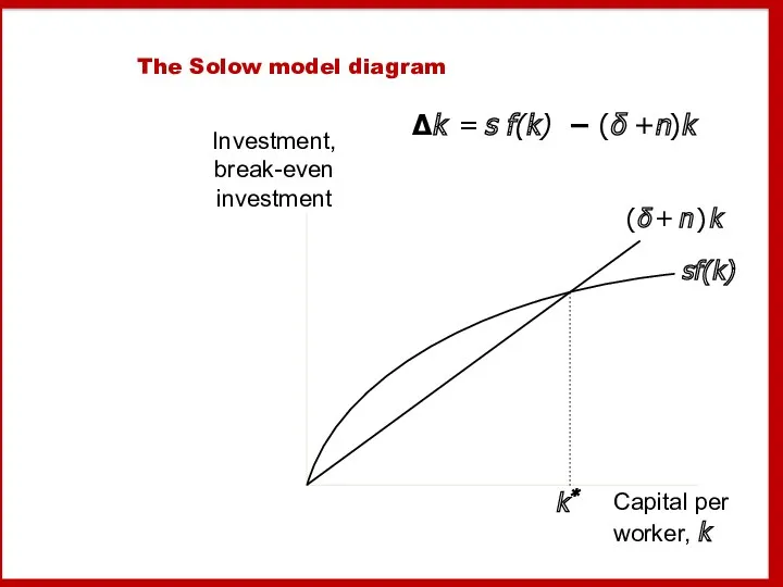
The Solow model diagram
Δk = s f(k) − (δ +n)k
The Solow model diagram
Δk = s f(k) − (δ +n)k
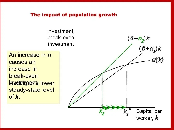
The impact of population growth
Investment, break-even investment
Capital per
worker, k
(δ
The impact of population growth
Investment, break-even investment
Capital per
worker, k
(δ
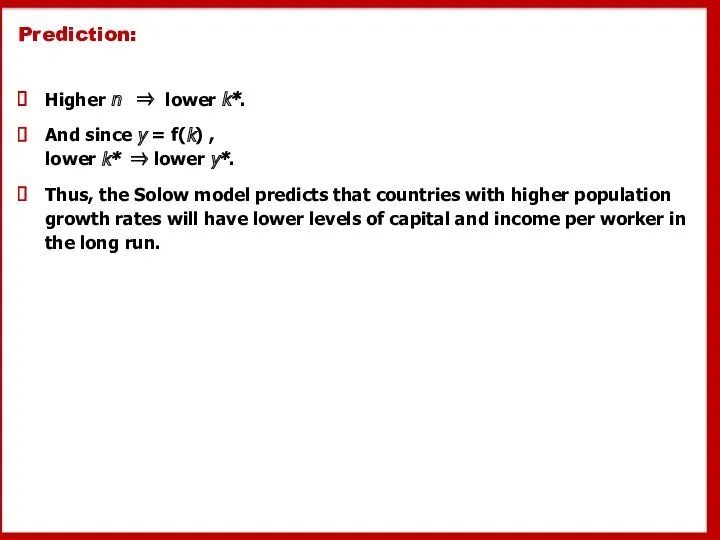
Prediction:
Higher n ⇒ lower k*.
And since y = f(k) ,
Prediction:
Higher n ⇒ lower k*.
And since y = f(k) ,
International evidence on population growth and income per person
100
1,000
10,000
100,000
0
1
2
3
4
5
Population Growth
(percent
International evidence on population growth and income per person
100
1,000
10,000
100,000
0
1
2
3
4
5
Population Growth
(percent
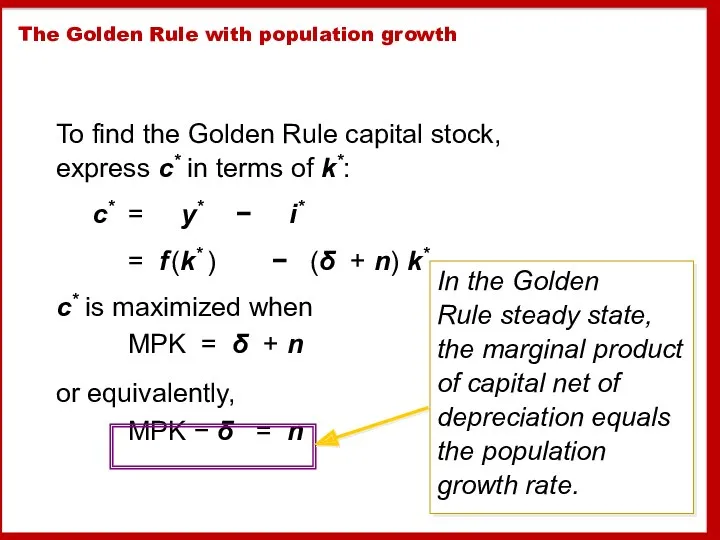
The Golden Rule with population growth
To find the Golden Rule capital
The Golden Rule with population growth
To find the Golden Rule capital
Alternative perspectives on population growth
The Malthusian Model (1798)
Predicts population growth will
Alternative perspectives on population growth
The Malthusian Model (1798)
Predicts population growth will
Alternative perspectives on population growth
The Kremerian Model (1993)
Posits that population growth
Alternative perspectives on population growth
The Kremerian Model (1993)
Posits that population growth
Chapter Summary
1. The Solow growth model shows that, in the long run,
Chapter Summary
1. The Solow growth model shows that, in the long run,
 Внешние эффекты (экстерналии)
 Обоснование ресурсов. Производственные мощности. Капитальные затраты. Затраты на сырье и материалы
 Экономика және оның қоғам өміріндегі орны
 Демография – наука о народонаселении
 Правовое и организационное обеспечение экономической безопасности
 Экономический рост и развитие
 Презентация Упражнения по теме спрос и предложение
 Статистические показатели, используемые в государственном регулировании
 Типи країн та показники їх економічного рівня
 Предмет и метод экономической теории. (Тема 1)
 Государственные и муниципальные унитарные предприятия. Производственные кооперативы. Объединения предприятий. Малый бизнес
 Историческое развитие человечества. Формационный подход
 Тема 9_Открытая экономика при несовершенной мобильности капитала
 Понятие, источники, элементы и показатели предпринимательского дохода
 Главная цель экономического развития региона Ленинградской области
 Занятие 29. Экономический рост
 Международные валютно-кредитные и финансовые организации и их регулирующая роль в мировом хозяйстве
 Занятие по Экономическому практикуму
 Рынок инноваций
 Развитие промышленности в Краснодарском крае
 Преступления в сфере экономической деятельности. Тема 21
 Сукупний попит та сукупна пропозиція: макроекономічна рівновага. (Тема 5)
 Технологічна політика ТНК
 Анализ технологических укладов
 Территория опережающего социально-экономического развития
 Риск и неопределенность
 Экономика семьи
 Экономика: наука и хозяйство