- The phillips curve, the natural rate of unemployment and inflation

Содержание
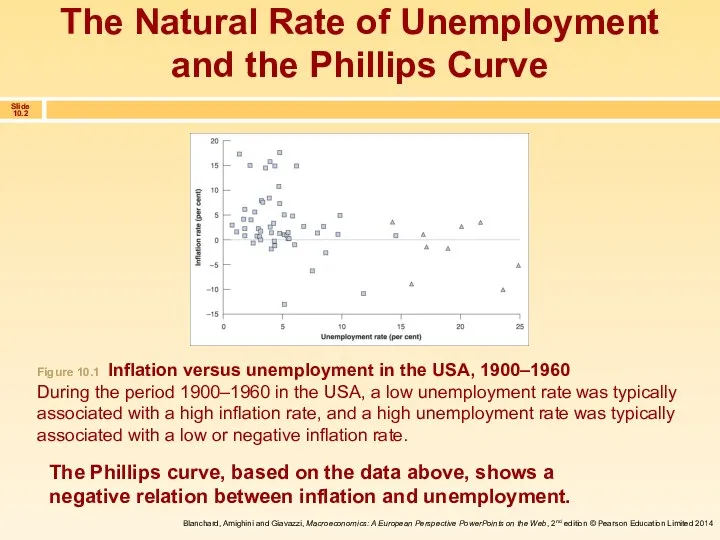
- 2. The Natural Rate of Unemployment and the Phillips Curve The Phillips curve, based on the data
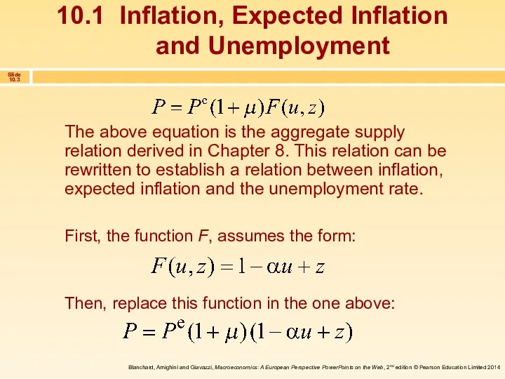
- 3. 10.1 Inflation, Expected Inflation and Unemployment The above equation is the aggregate supply relation derived in
- 4. The appendix to this chapter shows how to go from the equation above to the relation
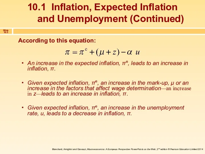
- 5. According to this equation: An increase in the expected inflation, πe, leads to an increase in
- 6. When referring to inflation, expected inflation or unemployment in a specific year, the equation above needs
- 7. If we set πte = 0, then: This is the negative relation between unemployment and inflation
- 8. The wage–price spiral: Given Low unemployment leads to a higher nominal wage. In response to the
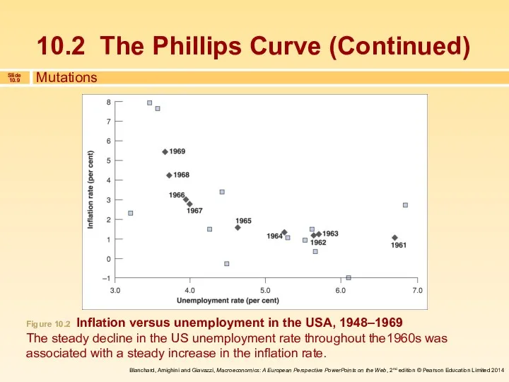
- 9. Mutations Figure 10.2 Inflation versus unemployment in the USA, 1948–1969 The steady decline in the US
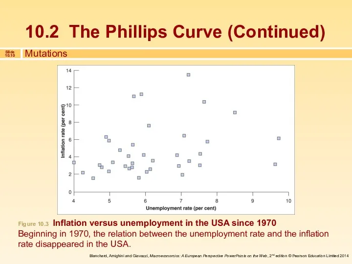
- 10. Mutations Figure 10.3 Inflation versus unemployment in the USA since 1970 Beginning in 1970, the relation
- 11. The negative relation between unemployment and inflation held throughout the 1960s, but it vanished after that
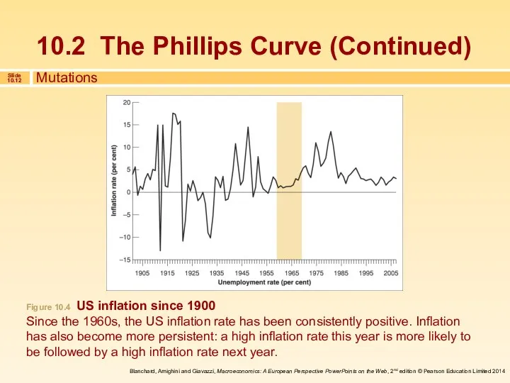
- 12. Mutations Figure 10.4 US inflation since 1900 Since the 1960s, the US inflation rate has been
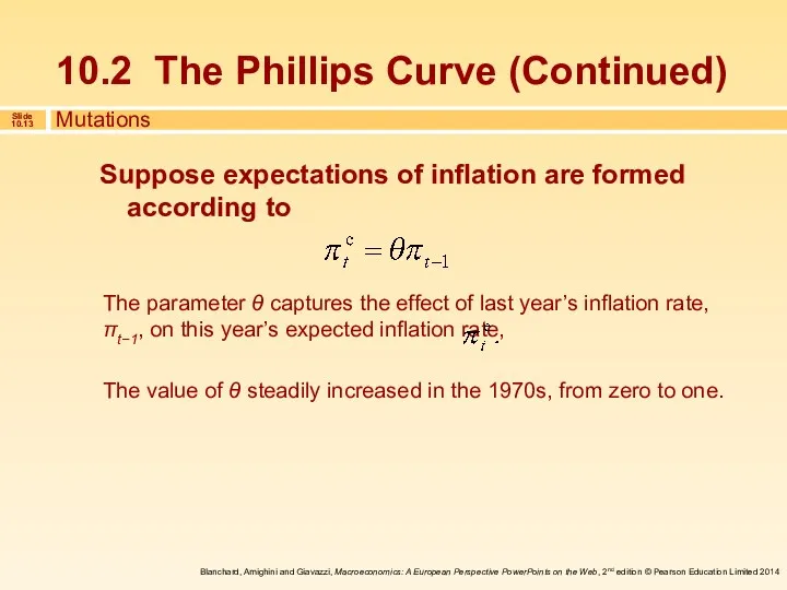
- 13. Suppose expectations of inflation are formed according to The parameter θ captures the effect of last
- 14. We can think of what happened in the 1970s as an increase in the value of
- 15. When θ equals zero, we get the original Phillips curve, a relation between the inflation rate
- 16. When θ = 1, the unemployment rate affects not the inflation rate, but the change in
- 17. The line that best fits the scatter of points for the period 1970–2006 is: Mutations Figure
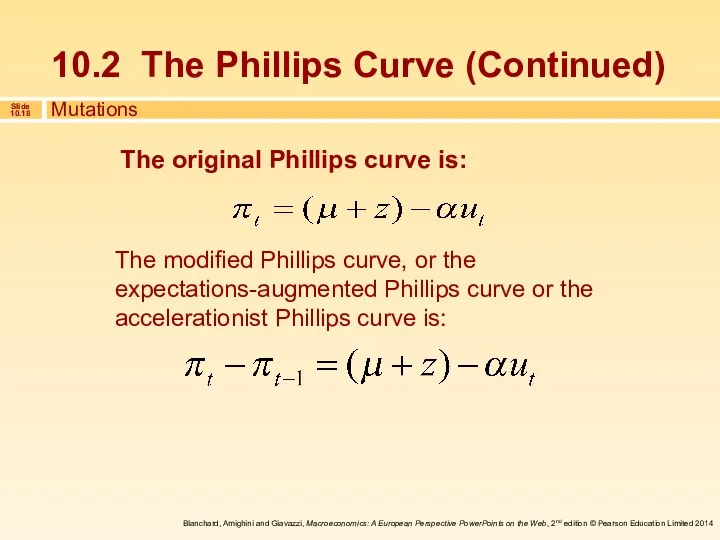
- 18. The original Phillips curve is: The modified Phillips curve, or the expectations-augmented Phillips curve or the
- 19. Friedman and Phelps questioned the trade-off between unemployment and inflation. They argued that the unemployment rate
- 20. This is an important relation because it gives another way of thinking about the Phillips curve
- 21. The equation above is an important relation for two reasons: It gives us another way of
- 22. Let’s summarize what we have learned so far: When the unemployment rate exceeds the natural rate
- 23. The factors that affect the natural rate of unemployment above differ across countries. Therefore, there is
- 24. In the equation above, the terms μ and z may not be constant but, in fact,
- 25. What explains European unemployment? Labour market rigidities: A generous system of unemployment insurance A high degree
- 26. The relation between unemployment and inflation is likely to change with the level and the persistence
- 27. Let λ denote the proportion of labour contracts that is indexed, and (1− λ) the proportion
- 29. Скачать презентацию
The Natural Rate of Unemployment
and the Phillips Curve
The Phillips curve, based
The Natural Rate of Unemployment
and the Phillips Curve
The Phillips curve, based
10.1 Inflation, Expected Inflation
and Unemployment
The above equation is the aggregate supply
10.1 Inflation, Expected Inflation
and Unemployment
The above equation is the aggregate supply
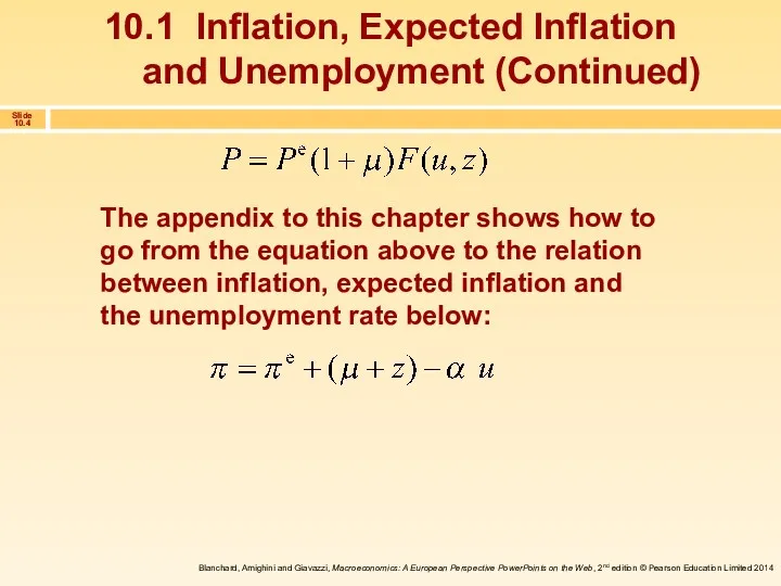
The appendix to this chapter shows how to go from the
The appendix to this chapter shows how to go from the
According to this equation:
An increase in the expected inflation, πe, leads
According to this equation:
An increase in the expected inflation, πe, leads
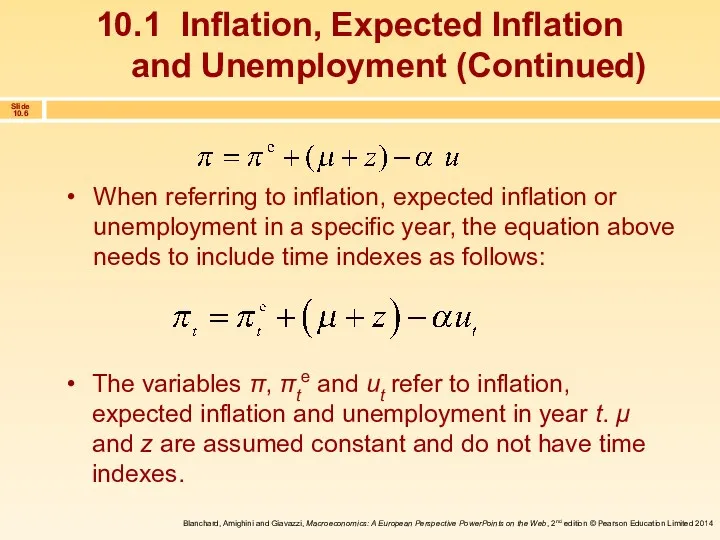
When referring to inflation, expected inflation or unemployment in a specific
When referring to inflation, expected inflation or unemployment in a specific
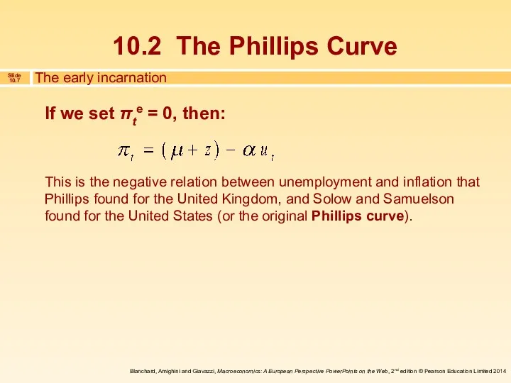
If we set πte = 0, then:
This is the negative relation
If we set πte = 0, then:
This is the negative relation
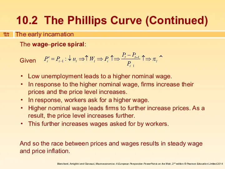
The wage–price spiral:
Given
Low unemployment leads to a higher nominal wage.
In
The wage–price spiral:
Given
Low unemployment leads to a higher nominal wage.
In
Mutations
Figure 10.2 Inflation versus unemployment in the USA, 1948–1969
The steady decline
Mutations
Figure 10.2 Inflation versus unemployment in the USA, 1948–1969 The steady decline
Mutations
Figure 10.3 Inflation versus unemployment in the USA since 1970
Beginning in
Mutations
Figure 10.3 Inflation versus unemployment in the USA since 1970 Beginning in
The negative relation between unemployment and inflation held throughout the 1960s,
The negative relation between unemployment and inflation held throughout the 1960s,
Mutations
Figure 10.4 US inflation since 1900
Since the 1960s, the US inflation
Mutations
Figure 10.4 US inflation since 1900 Since the 1960s, the US inflation
Suppose expectations of inflation are formed according to
The parameter θ captures
Suppose expectations of inflation are formed according to
The parameter θ captures
We can think of what happened in the 1970s as an
We can think of what happened in the 1970s as an
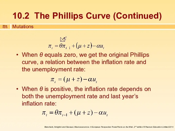
When θ equals zero, we get the original Phillips curve, a
When θ equals zero, we get the original Phillips curve, a
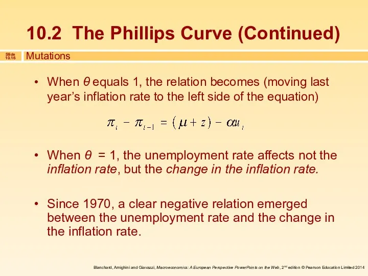
When θ = 1, the unemployment rate affects not the inflation
When θ = 1, the unemployment rate affects not the inflation
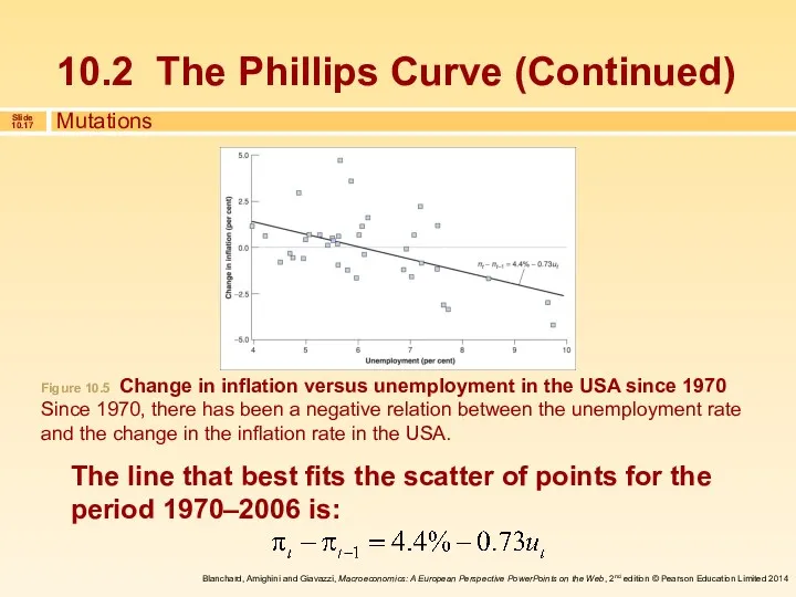
The line that best fits the scatter of points for the
The line that best fits the scatter of points for the
The original Phillips curve is:
The modified Phillips curve, or the expectations-augmented
The original Phillips curve is:
The modified Phillips curve, or the expectations-augmented
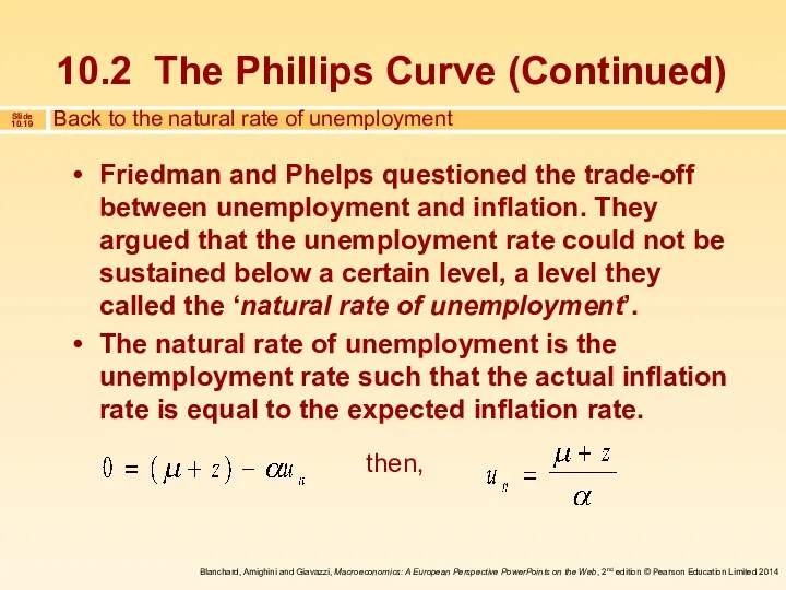
Friedman and Phelps questioned the trade-off between unemployment and inflation. They
Friedman and Phelps questioned the trade-off between unemployment and inflation. They
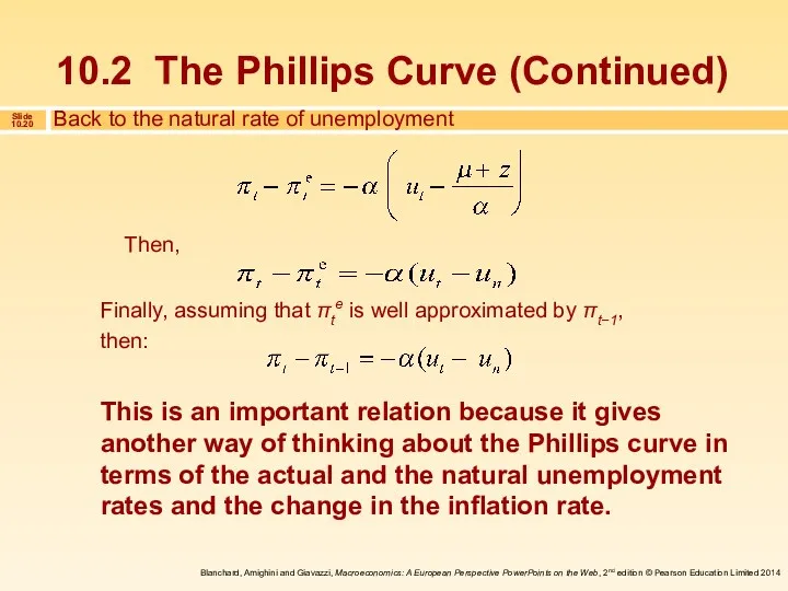
This is an important relation because it gives another way of
This is an important relation because it gives another way of
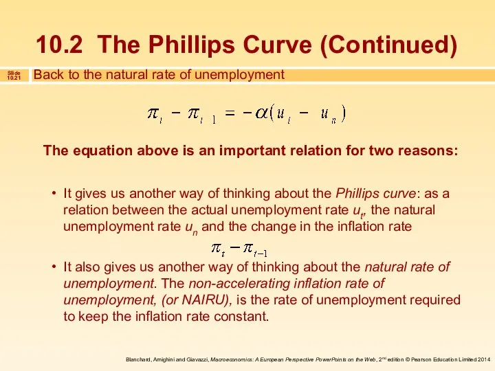
The equation above is an important relation for two reasons:
It gives
The equation above is an important relation for two reasons:
It gives
Let’s summarize what we have learned so far:
When the unemployment rate
Let’s summarize what we have learned so far:
When the unemployment rate
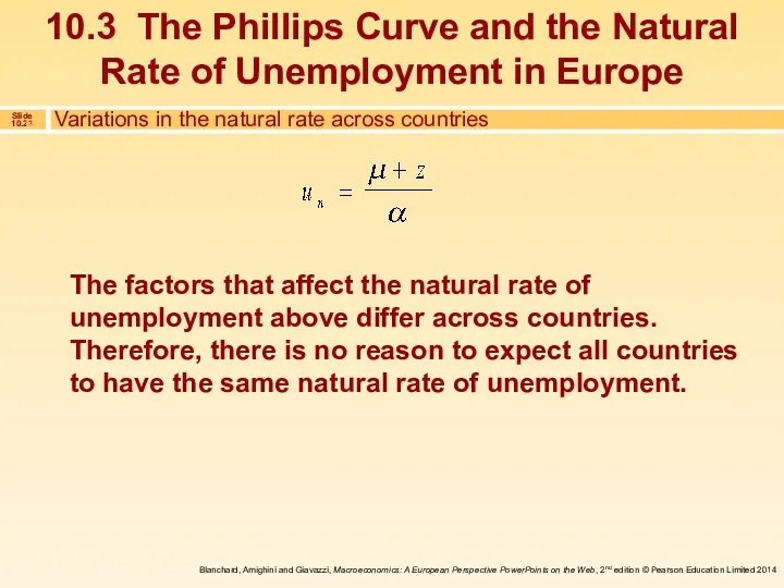
The factors that affect the natural rate of unemployment above differ
The factors that affect the natural rate of unemployment above differ
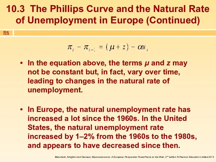
In the equation above, the terms μ and z may not
In the equation above, the terms μ and z may not

What explains European unemployment?
Labour market rigidities:
A generous system of unemployment insurance
A
What explains European unemployment?
Labour market rigidities:
A generous system of unemployment insurance
A
The relation between unemployment and inflation is likely to change with
The relation between unemployment and inflation is likely to change with
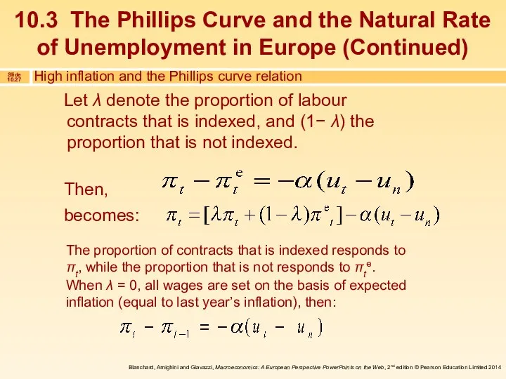
Let λ denote the proportion of labour contracts that is indexed,
Let λ denote the proportion of labour contracts that is indexed,
 Внешние эффекты (экстерналии)
 Обоснование ресурсов. Производственные мощности. Капитальные затраты. Затраты на сырье и материалы
 Экономика және оның қоғам өміріндегі орны
 Демография – наука о народонаселении
 Правовое и организационное обеспечение экономической безопасности
 Экономический рост и развитие
 Презентация Упражнения по теме спрос и предложение
 Статистические показатели, используемые в государственном регулировании
 Типи країн та показники їх економічного рівня
 Предмет и метод экономической теории. (Тема 1)
 Государственные и муниципальные унитарные предприятия. Производственные кооперативы. Объединения предприятий. Малый бизнес
 Историческое развитие человечества. Формационный подход
 Тема 9_Открытая экономика при несовершенной мобильности капитала
 Понятие, источники, элементы и показатели предпринимательского дохода
 Главная цель экономического развития региона Ленинградской области
 Занятие 29. Экономический рост
 Международные валютно-кредитные и финансовые организации и их регулирующая роль в мировом хозяйстве
 Занятие по Экономическому практикуму
 Рынок инноваций
 Развитие промышленности в Краснодарском крае
 Преступления в сфере экономической деятельности. Тема 21
 Сукупний попит та сукупна пропозиція: макроекономічна рівновага. (Тема 5)
 Технологічна політика ТНК
 Анализ технологических укладов
 Территория опережающего социально-экономического развития
 Риск и неопределенность
 Экономика семьи
 Экономика: наука и хозяйство