- The Small Open Economy

Содержание
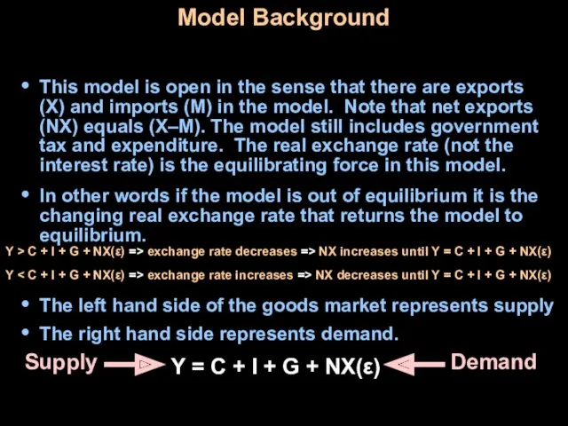
- 2. Model Background This model is open in the sense that there are exports (X) and imports
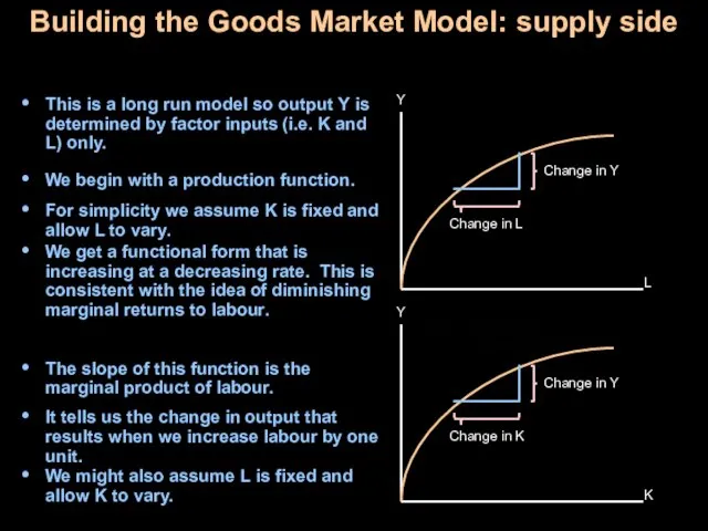
- 3. Building the Goods Market Model: supply side This is a long run model so output Y
- 4. If we chose to combine these images we would get a surface with output on the
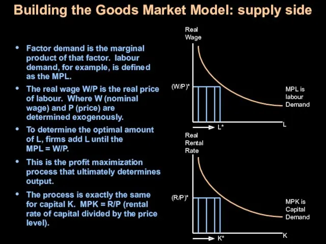
- 5. Building the Goods Market Model: supply side Factor demand is the marginal product of that factor.
- 6. Building the Goods Market Model: demand side We begin with consumption, investment, government expenditure, and net
- 7. Goods Market Equilibrium: The Loanable Funds Market We said the small open economy model long run
- 8. The Markets in Transition There are various effects which can enter the model and change either
- 10. Скачать презентацию
Model Background
This model is open in the sense that there are
Model Background
This model is open in the sense that there are
Building the Goods Market Model: supply side
This is a long run
Building the Goods Market Model: supply side
This is a long run
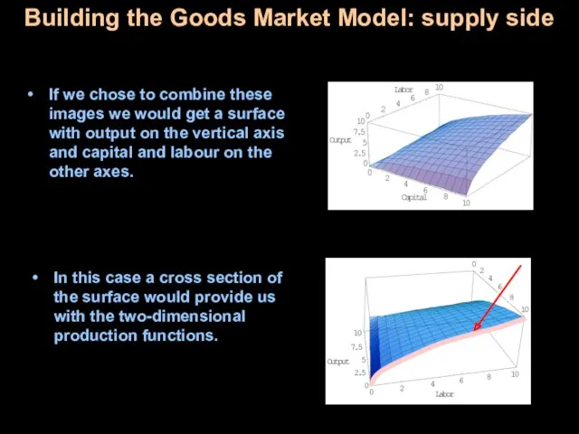
If we chose to combine these images we would get a
If we chose to combine these images we would get a
Building the Goods Market Model: supply side
Factor demand is the marginal
Building the Goods Market Model: supply side
Factor demand is the marginal

Building the Goods Market Model: demand side
We begin with consumption, investment,
Building the Goods Market Model: demand side
We begin with consumption, investment,
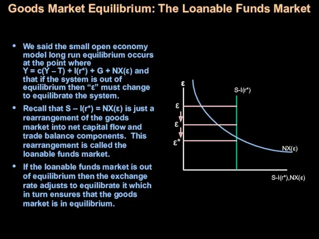
Goods Market Equilibrium: The Loanable Funds Market
We said the small
Goods Market Equilibrium: The Loanable Funds Market
We said the small
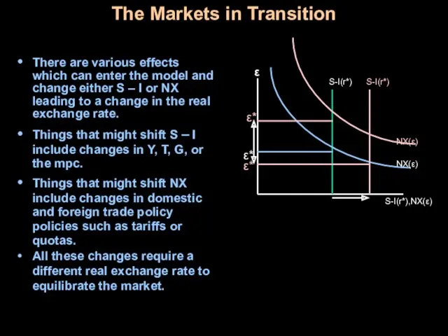
The Markets in Transition
There are various effects which can enter
The Markets in Transition
There are various effects which can enter
 Государственное регулирование экономики и его методы
 Основы теории риска проектов
 Оценка качества работы управляющих организаций за I полугодие 2017
 Экономика семьи
 Постсоветское пространство. Укрепление влияния России и его кризис
 Економіка національного господарства. Основні характеристики і особливості розвитку. (Тема 1)
 Бюджетное ограничение. Равновесие потребителя
 ЕГЭ по Обществознанию.Экономика
 Экономика предприятия НГК. Практикум Расчет сметы затрат и калькуляция затрат на производство нефтепродуктов
 Проблемы экономики России и ее регионов (анализ тенденций и прогноз развития экономики Ветлужского района на 2018 год)
 Теория отраслевых рынков
 Швеция в мировой экономике
 Рыночная экономика
 Фискальная и монетарная политика. Инструменты государственной макроэкономической политики
 Сельское хозяйство Израиля
 Тың игеру және тыңайған жерлерді игеру
 Международные транспортные коридоры
 Мировая экономика и внешняя торговля
 Большие (технологические) циклы Н. Д. Кондратьева. Технологический уклад (С. Ю. Глазьев)
 Методи експертного оцінювання. (Лекція 8)
 Нефтяная промышленность
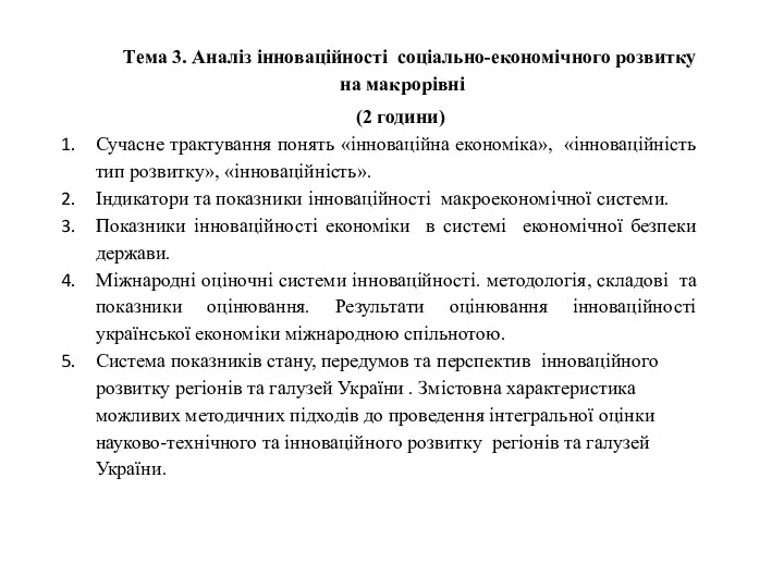 Аналіз інноваційності соціально-економічного розвитку на макрорівні
 Заработная плата и её виды. Профессии. Карьера
 Джон Мейнард Кейнс
 Финансовая экономика. Мировая экономика и международные экономические отношения
 Производственная структура предприятия
 Учет затрат на производство продукции отрасли растениеводства ООО ФХ Макаркова А.М.
 Система национальных счетов и основные макроэкономические показатели