- 1D PIC code for TwoStream Plasma Instability

Содержание
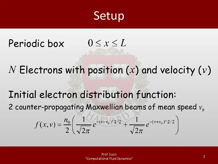
- 2. Setup Prof. Succi "Computational Fluid Dynamics" Periodic box Initial electron distribution function: 2 counter-propagating Maxwellian beams
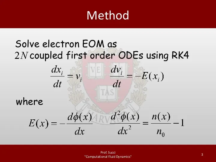
- 3. Method Prof. Succi "Computational Fluid Dynamics" Solve electron EOM as coupled first order ODEs using RK4
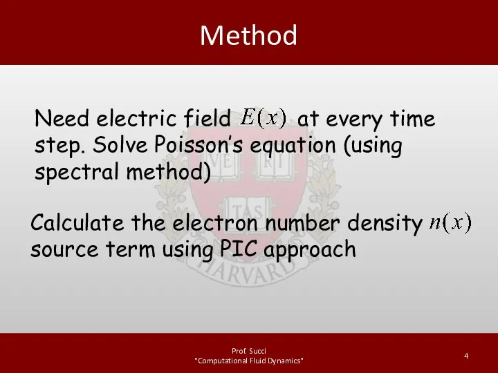
- 4. Method Prof. Succi "Computational Fluid Dynamics" Need electric field at every time step. Solve Poisson’s equation
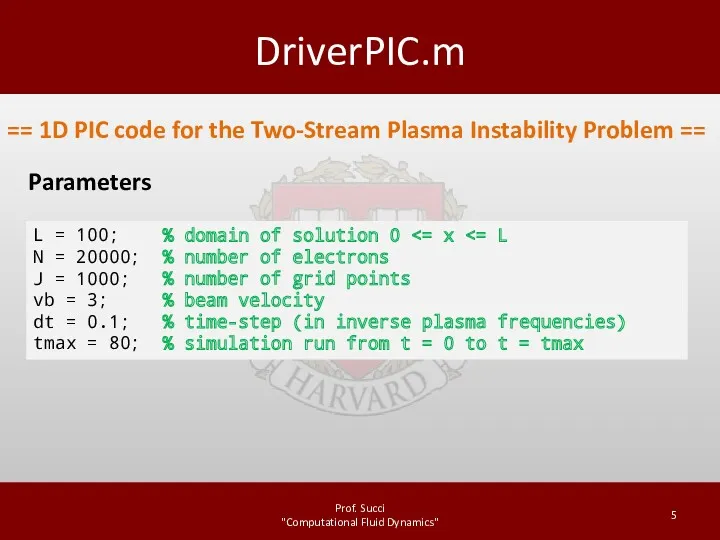
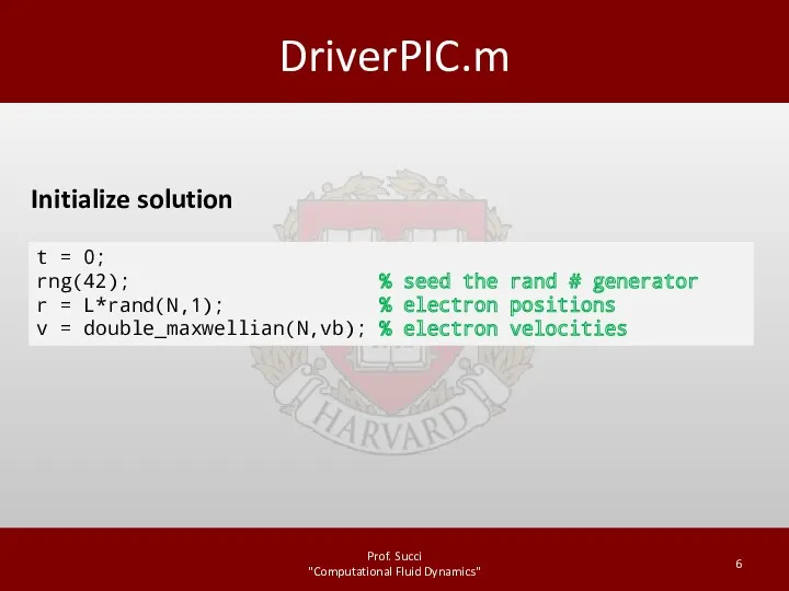
- 5. DriverPIC.m Prof. Succi "Computational Fluid Dynamics" == 1D PIC code for the Two-Stream Plasma Instability Problem
- 6. DriverPIC.m Prof. Succi "Computational Fluid Dynamics" t = 0; rng(42); % seed the rand # generator
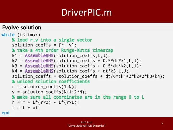
- 7. DriverPIC.m Prof. Succi "Computational Fluid Dynamics" while (t % load r,v into a single vector solution_coeffs
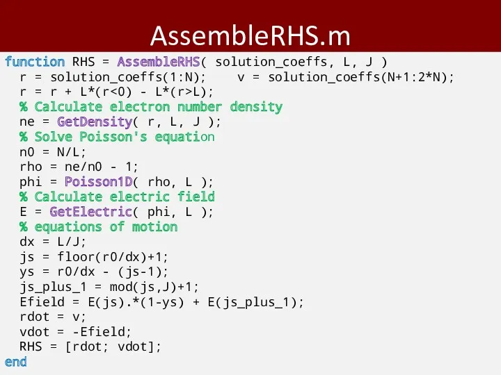
- 8. AssembleRHS.m Prof. Succi "Computational Fluid Dynamics" function RHS = AssembleRHS( solution_coeffs, L, J ) r =
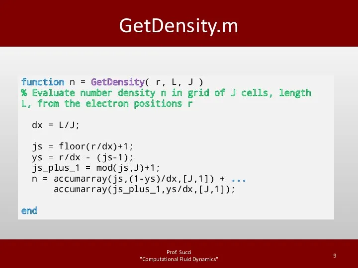
- 9. GetDensity.m Prof. Succi "Computational Fluid Dynamics" function n = GetDensity( r, L, J ) % Evaluate
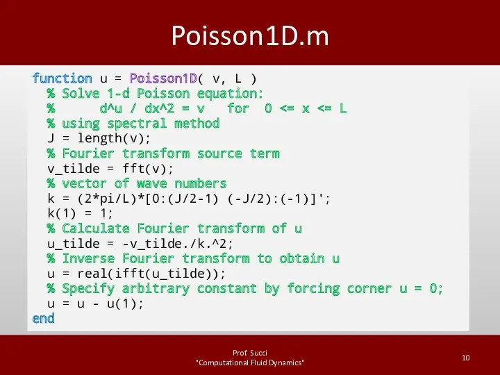
- 10. Poisson1D.m Prof. Succi "Computational Fluid Dynamics" function u = Poisson1D( v, L ) % Solve 1-d
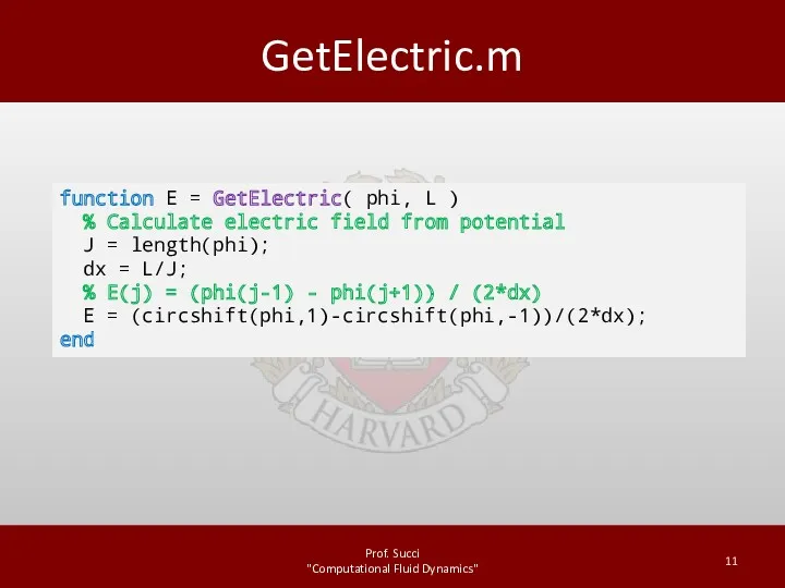
- 11. GetElectric.m Prof. Succi "Computational Fluid Dynamics" function E = GetElectric( phi, L ) % Calculate electric
- 13. Скачать презентацию
Setup
Prof. Succi "Computational Fluid Dynamics"
Periodic box
Initial electron distribution function:
2 counter-propagating Maxwellian
Setup
Prof. Succi "Computational Fluid Dynamics"
Periodic box
Initial electron distribution function:
2 counter-propagating Maxwellian
Method
Prof. Succi "Computational Fluid Dynamics"
Solve electron EOM as
coupled first order
Method
Prof. Succi "Computational Fluid Dynamics"
Solve electron EOM as
coupled first order
Method
Prof. Succi "Computational Fluid Dynamics"
Need electric field at every time step.
Method
Prof. Succi "Computational Fluid Dynamics"
Need electric field at every time step.
DriverPIC.m
Prof. Succi "Computational Fluid Dynamics"
== 1D PIC code for the Two-Stream
DriverPIC.m
Prof. Succi "Computational Fluid Dynamics"
== 1D PIC code for the Two-Stream
DriverPIC.m
Prof. Succi "Computational Fluid Dynamics"
t = 0;
rng(42); % seed the rand
DriverPIC.m
Prof. Succi "Computational Fluid Dynamics"
t = 0;
rng(42); % seed the rand
DriverPIC.m
Prof. Succi "Computational Fluid Dynamics"
while (t<=tmax)
% load r,v into a
DriverPIC.m
Prof. Succi "Computational Fluid Dynamics"
while (t<=tmax)
% load r,v into a
AssembleRHS.m
Prof. Succi "Computational Fluid Dynamics"
function RHS = AssembleRHS( solution_coeffs, L, J
AssembleRHS.m
Prof. Succi "Computational Fluid Dynamics"
function RHS = AssembleRHS( solution_coeffs, L, J
GetDensity.m
Prof. Succi "Computational Fluid Dynamics"
function n = GetDensity( r, L, J
GetDensity.m
Prof. Succi "Computational Fluid Dynamics"
function n = GetDensity( r, L, J
Poisson1D.m
Prof. Succi "Computational Fluid Dynamics"
function u = Poisson1D( v, L )
Poisson1D.m
Prof. Succi "Computational Fluid Dynamics"
function u = Poisson1D( v, L )
GetElectric.m
Prof. Succi "Computational Fluid Dynamics"
function E = GetElectric( phi, L )
GetElectric.m
Prof. Succi "Computational Fluid Dynamics"
function E = GetElectric( phi, L )
 Законы геометрической оптики
 Физика пласта
 Элементарные частицы
 урок-обобщение: Газовые законы
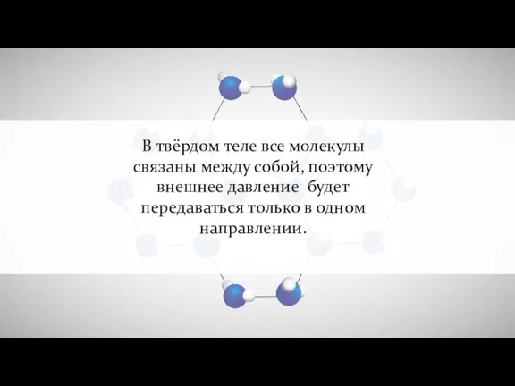 Передача давления жидкостями и газами. Закон Паскаля
 Полупроводниковые дозиметрические детекторы
 Свайные фундаменты. Классификация. (Лекция 6)
 Виды сил
 Конструкция и техническое обслуживание пассажирских вагонов
 Kosmicheskoe-izluchenie
 Учебный проект по теме Виды теплопередачи
 Карданная передача
 Презетанция Ток в вакууме
 Термическая стабильность структуры наноматериалов
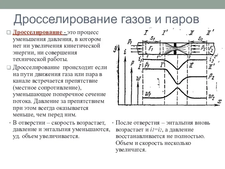 Дросселирование газов и паров
 Явление электромагнитной индукции
 Спектральные характеристики одномерных и трехмерных жидкокристаллических фотонных кристаллов
 Лекция № 1. Механические характеристики асинхронных электродвигателей
 Занятие спецкурса о физике в 8 классе Бионика и электрические явления в живой природе
 Властивості рідин. Поверхневий натяг. Змочування
 Відновлення деталей електролітичними способами. Зміцнення поверхонь
 Толық тізбек үшін Ом заңы
 Кузнечно-сварочная практика. Специальность 190604 Техническое обслуживание и ремонт автомобильного транспорта
 Физико-технические основы электроэнергетики. Лекция 10
 Модульные технологии как технологии здоровьесбережения.
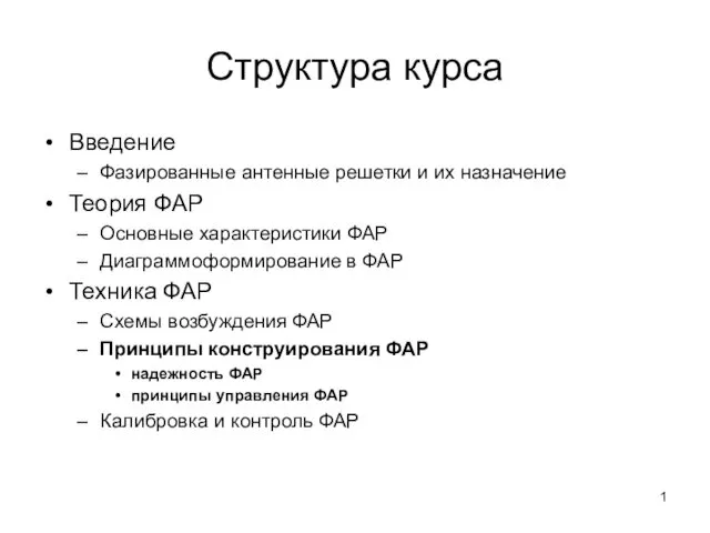 Фазированные антенные решетки и их назначение. Надежность ФАР
 Радиоактивность
 Подшипники качения