- Control systems

Содержание
- 2. By failing to prepare, you are preparing to fail. Benjamin Franklin
- 3. Contents -Review of Previous Lectures -System Response Analysis
- 4. Review Once transfer function is obtained, we can start to analyze the response of the system
- 5. Review-Block Diagram Three Elementary Block Diagrams Series connection Parallel connection Negative Feedback connection
- 6. Negative feedback :Single-loop gain The gain of a single-loop negative feedback system is given by the
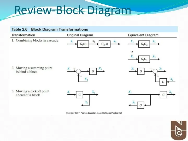
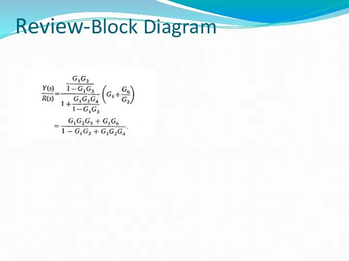
- 7. Review-Block Diagram
- 8. Table 2.6 (continued) Block Diagram Transformations Review-Block Diagram
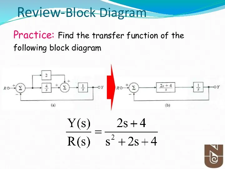
- 9. Review-Block Diagram Practice: Find the transfer function of the following block diagram
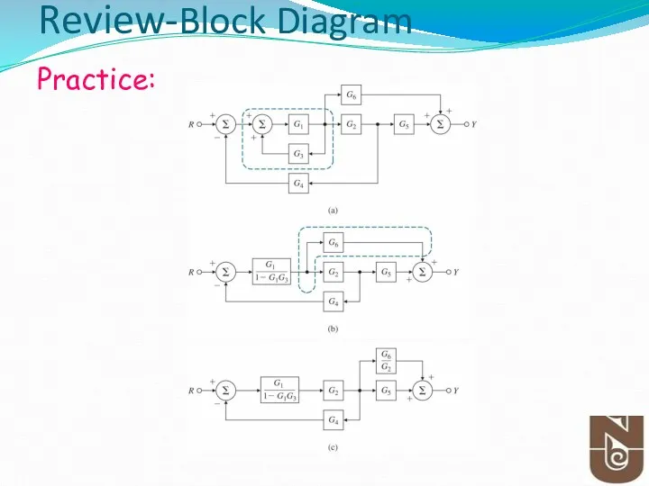
- 10. Review-Block Diagram Practice:
- 11. Review-Block Diagram
- 12. Time domain and frequency domain
- 17. Poles and Zeros K is the transfer gain The roots of numerator is called zeros of
- 18. System Response: Complex system
- 19. System Response: Stability in s-plane
- 20. Key points: Effect of Poles and Zeros
- 21. Example: Consider the following transfer function Determine: Poles and Zeros? System Response
- 22. System Response: Effect of pole location
- 23. Example: Consider the following transfer function Determine: Poles and Zeros? System Response
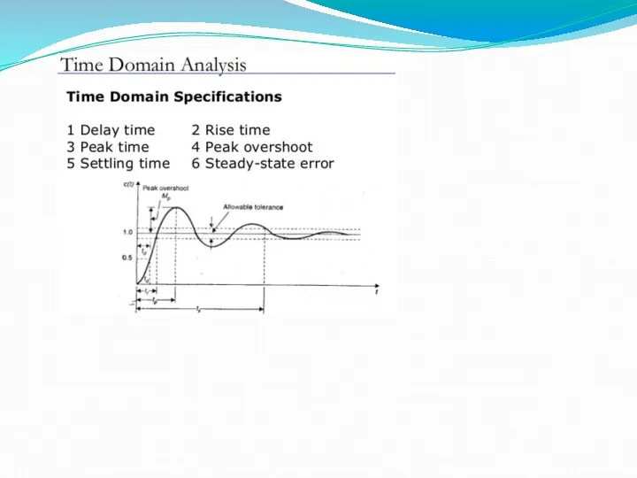
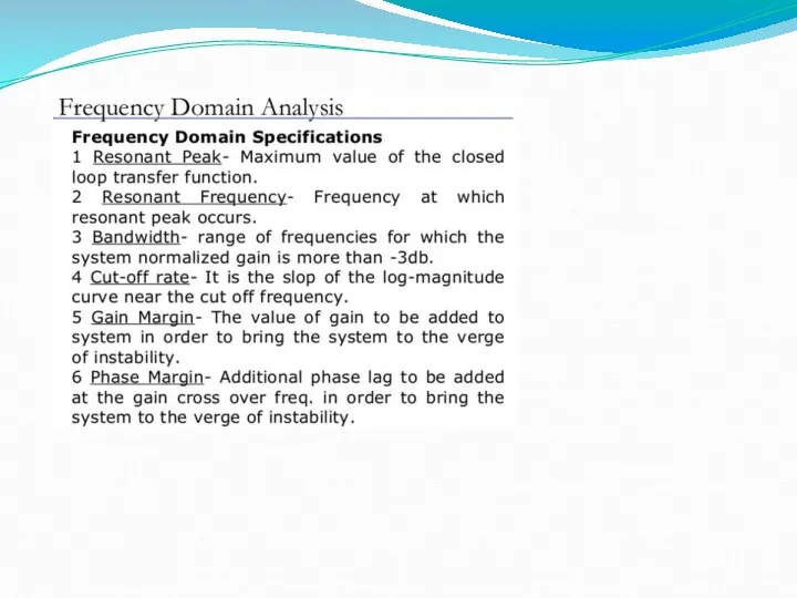
- 24. Time-Domain Specification To measure the performance of a system we use standard test input signals. This
- 25. Time-Domain Specification Test Input Signals step input ramp input parabolic input The step input is the
- 26. Time-Domain Specification Example The transfer function: The system response to a unit step input (A=1):
- 27. System Response Example 2: Consider the following transfer function Determine: impulse response
- 28. First Order System Response
- 29. Example 1: Consider the following transfer function Determine: impulse response(response when r(t) is impulse function) Classify
- 30. First Order System Response- Impulse response
- 31. Let us consider the following closed-loop system: The TF of the closed-loop system: Utilizing the general
- 32. Standard Second Order System
- 33. Figure 3.24 Graphs of regions in the s-plane delineated by certain transient requirements: (a) rise time;
- 34. Transformation of the specification to the s-plane Example 3.25 Find allowable regions in the s-plane for
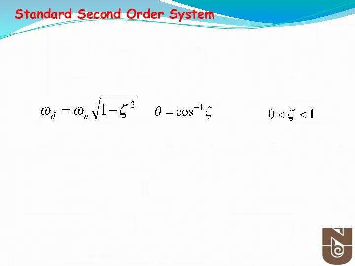
- 35. Mp? Standard Second Order System
- 36. Poles (roots) location of the second order complex system. Standard Second Order System Standard Second Order
- 37. Classification of Type Response of 2nd Order Systems Undamped: ζ=0 Under-damped: 0 Critical damped: ζ=1 Over-damped:
- 38. As ζ decreases, the response becomes increasingly oscillatory. Standard Second Order System
- 39. Time-Domain Specification Standard performance measures are usually defined in term of the step response of a
- 40. Time-Domain Specification Standard performance measures are usually defined in term of the step response of a
- 41. Time-Domain Specification -Rise Time, Tr- A precise analytical relationship between rise time and damping ratio ζ
- 42. Time-Domain Specification Maximum overshoot (in percentage) is defined as -Maximum Overshoot, Mp
- 43. Time-Domain Specification Tp is found by differentiating y(t) and finding the first zero crossing after t=0.
- 44. Time-Domain Specification -Settling Time Ts- For a second order system, we seek to determine the time
- 45. Time-Domain Specification Exercise # 1 Find Tr, Tp, Mp and Ts for the following transfer function:
- 46. Time-Domain Specification Exercise # 2 Find Tr, Tp, Mp and Ts for the following transfer function:
- 47. Exercise # 3 If the system response requirements are tr = 0.6, Mp = 10% and
- 48. Exercise # 4 Problem# If the system response requirements are tr = 0.6, Mp = 10%
- 49. Time-Domain Specification Exercise # 5 Find Tr, Tp, Mp and Ts for the following transfer function:
- 50. Time-Domain Specification Exercise # 6 Find Tr, Tp, Mp and Ts for the following transfer function:
- 51. Time-Domain Specification Exercise # 7 Find Tr, Tp, Mp and Ts for the following transfer function:
- 52. Figure - Multiple-loop feedback control system. Example - Block diagram Find TF from the given block
- 53. Figure 2.27 Block diagram reduction of the system of Figure 2.26. Quiz # 4- Answer to
- 54. System Response Consider the following transfer function Determine: i) Impulse response graphically ii) Classify stability Find
- 55. Impulse response Answer
- 56. Midterm Exam March 4, 2016, Friday, Time:8.00-9.00 Venue-6.141 & 5.103 Topics- Cover Until February
- 58. Tell me, I will forget! Show me, I may remember! Involve me, I will understand! Benjamin
- 60. Скачать презентацию

By failing to prepare, you are preparing to fail.
Benjamin Franklin
By failing to prepare, you are preparing to fail.
Benjamin Franklin
Contents
-Review of Previous Lectures
-System Response Analysis
Contents
-Review of Previous Lectures
-System Response Analysis
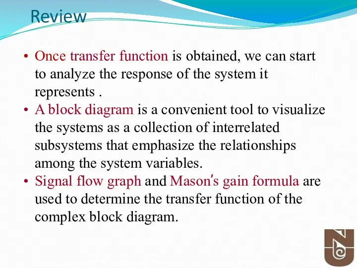
Review
Once transfer function is obtained, we can start to analyze the
Review
Once transfer function is obtained, we can start to analyze the
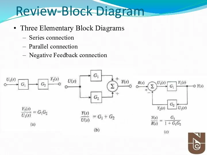
Review-Block Diagram
Three Elementary Block Diagrams
Series connection
Parallel connection
Negative Feedback connection
Review-Block Diagram
Three Elementary Block Diagrams
Series connection
Parallel connection
Negative Feedback connection
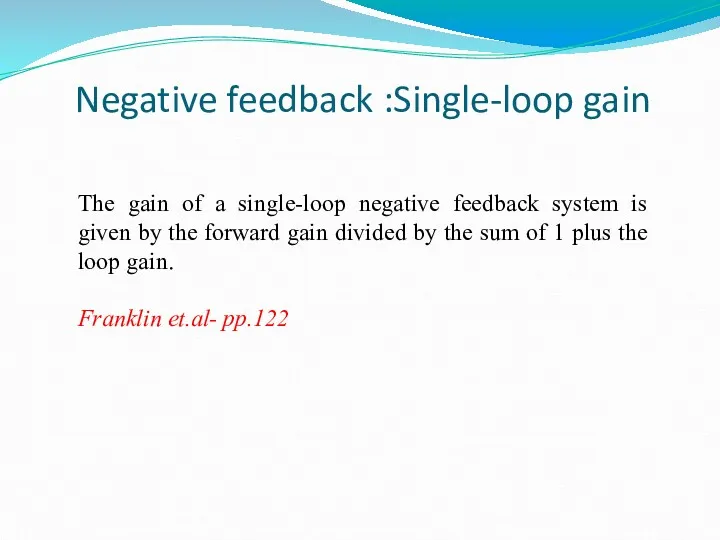
Negative feedback :Single-loop gain
The gain of a single-loop negative feedback system
Negative feedback :Single-loop gain
The gain of a single-loop negative feedback system
Review-Block Diagram
Review-Block Diagram
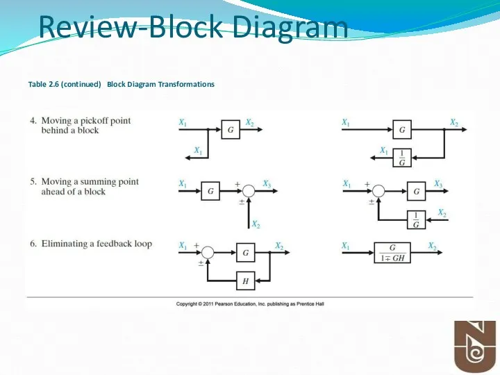
Table 2.6 (continued) Block Diagram Transformations
Review-Block Diagram
Table 2.6 (continued) Block Diagram Transformations
Review-Block Diagram
Review-Block Diagram
Practice: Find the transfer function of the following block diagram
Review-Block Diagram
Practice: Find the transfer function of the following block diagram
Review-Block Diagram
Practice:
Review-Block Diagram
Practice:
Review-Block Diagram
Review-Block Diagram
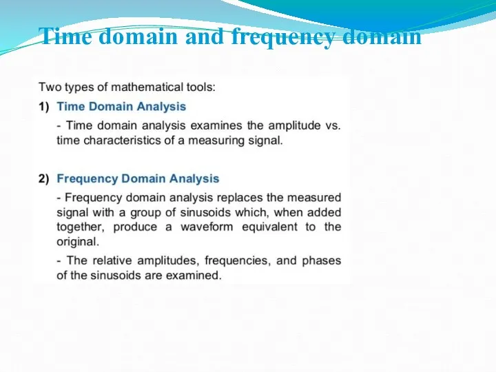
Time domain and frequency domain
Time domain and frequency domain

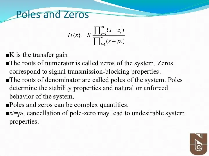
Poles and Zeros
K is the transfer gain
The roots of numerator is
Poles and Zeros
K is the transfer gain
The roots of numerator is
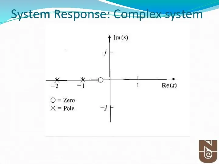
System Response: Complex system
System Response: Complex system
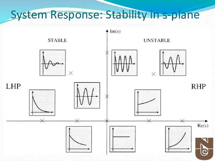
System Response: Stability in s-plane
System Response: Stability in s-plane
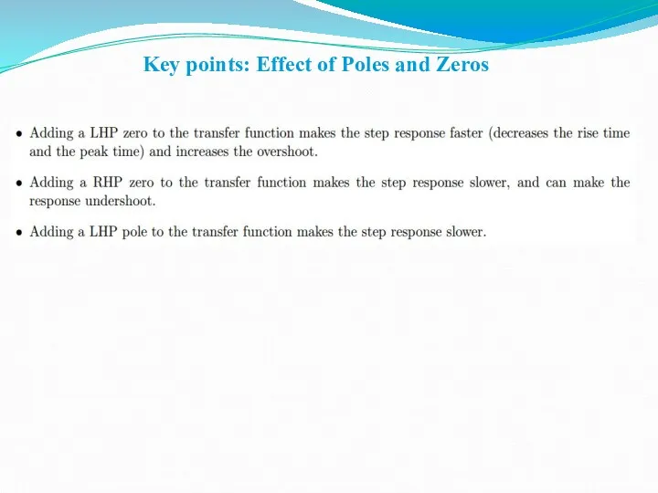
Key points: Effect of Poles and Zeros
Key points: Effect of Poles and Zeros
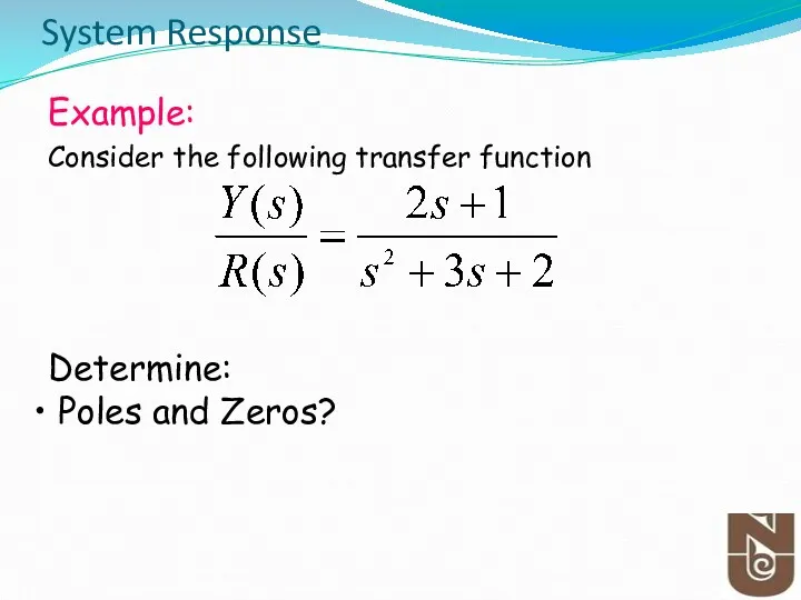
Example:
Consider the following transfer function
Determine:
Poles and Zeros?
System Response
Example:
Consider the following transfer function
Determine:
Poles and Zeros?
System Response
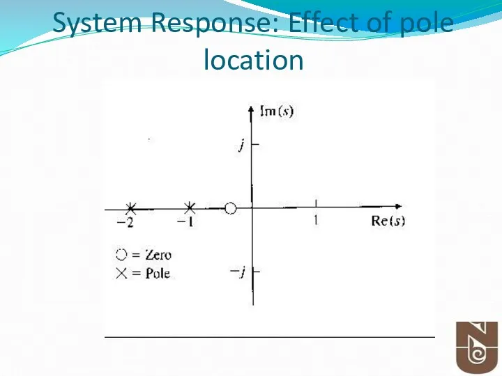
System Response: Effect of pole location
System Response: Effect of pole location
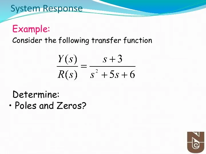
Example:
Consider the following transfer function
Determine:
Poles and Zeros?
System Response
Example:
Consider the following transfer function
Determine:
Poles and Zeros?
System Response
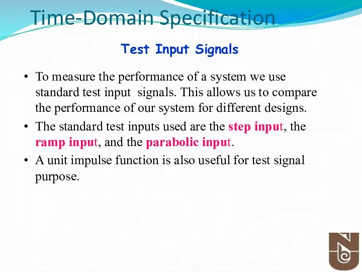
Time-Domain Specification
To measure the performance of a system we use standard
Time-Domain Specification
To measure the performance of a system we use standard
Time-Domain Specification
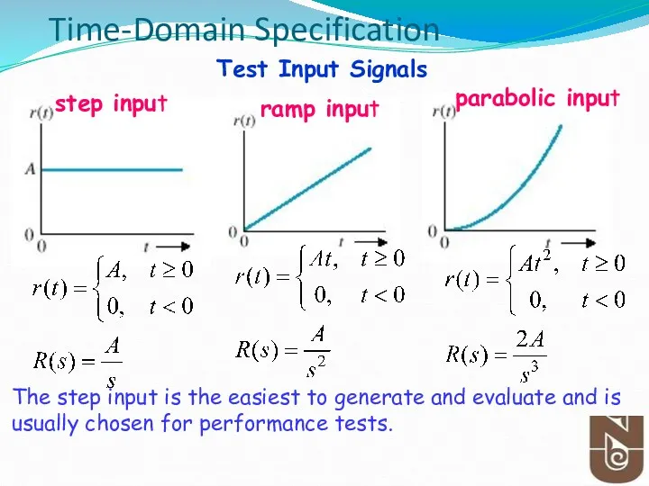
Test Input Signals
step input
ramp input
parabolic input
The step input is the
Time-Domain Specification
Test Input Signals
step input
ramp input
parabolic input
The step input is the
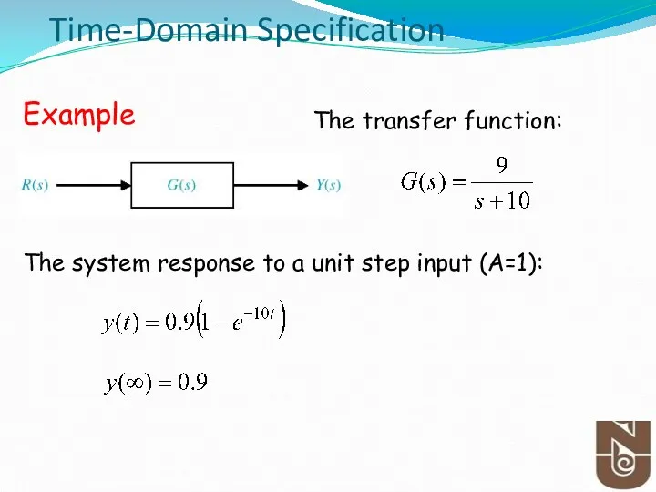
Time-Domain Specification
Example
The transfer function:
The system response to a unit step input
Time-Domain Specification
Example
The transfer function:
The system response to a unit step input
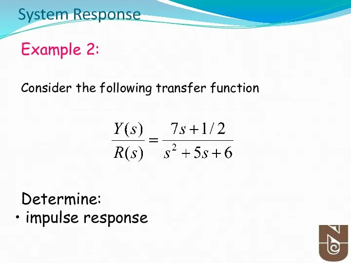
System Response
Example 2:
Consider the following transfer function
Determine:
impulse response
System Response
Example 2:
Consider the following transfer function
Determine:
impulse response

First Order System Response
First Order System Response
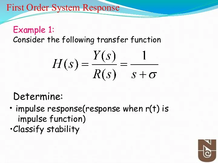
Example 1:
Consider the following transfer function
Determine:
impulse response(response when r(t) is
Example 1:
Consider the following transfer function
Determine:
impulse response(response when r(t) is
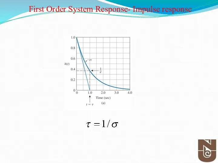
First Order System Response- Impulse response
First Order System Response- Impulse response
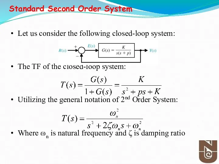
Let us consider the following closed-loop system:
The TF of the closed-loop
Let us consider the following closed-loop system:
The TF of the closed-loop
Standard Second Order System
Standard Second Order System
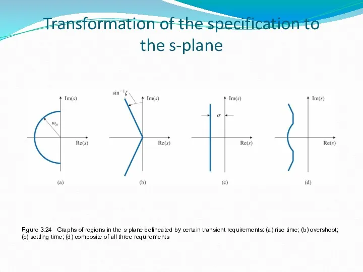
Figure 3.24 Graphs of regions in the s-plane delineated by certain
Figure 3.24 Graphs of regions in the s-plane delineated by certain
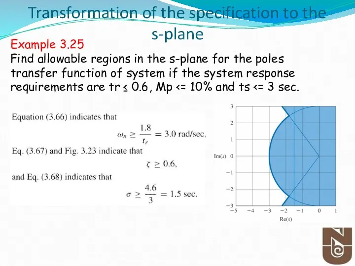
Transformation of the specification to the s-plane
Example 3.25
Find allowable regions in
Transformation of the specification to the s-plane
Example 3.25
Find allowable regions in
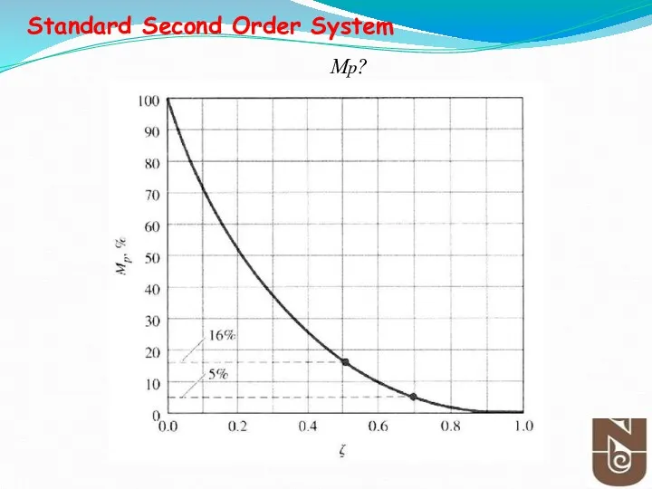
Mp?
Standard Second Order System
Mp?
Standard Second Order System
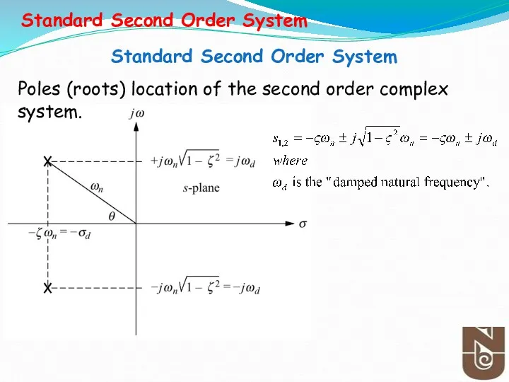
Poles (roots) location of the second order complex system.
Standard Second Order
Poles (roots) location of the second order complex system.
Standard Second Order

Classification of Type Response of 2nd Order Systems
Undamped: ζ=0
Under-damped: 0<ζ<1
Critical damped:
Classification of Type Response of 2nd Order Systems
Undamped: ζ=0
Under-damped: 0<ζ<1
Critical damped:
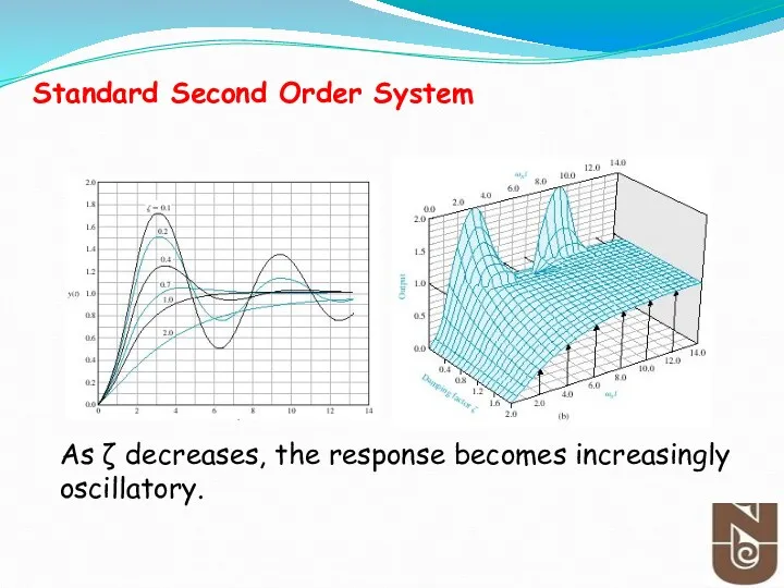
As ζ decreases, the response becomes increasingly oscillatory.
Standard Second Order System
As ζ decreases, the response becomes increasingly oscillatory.
Standard Second Order System
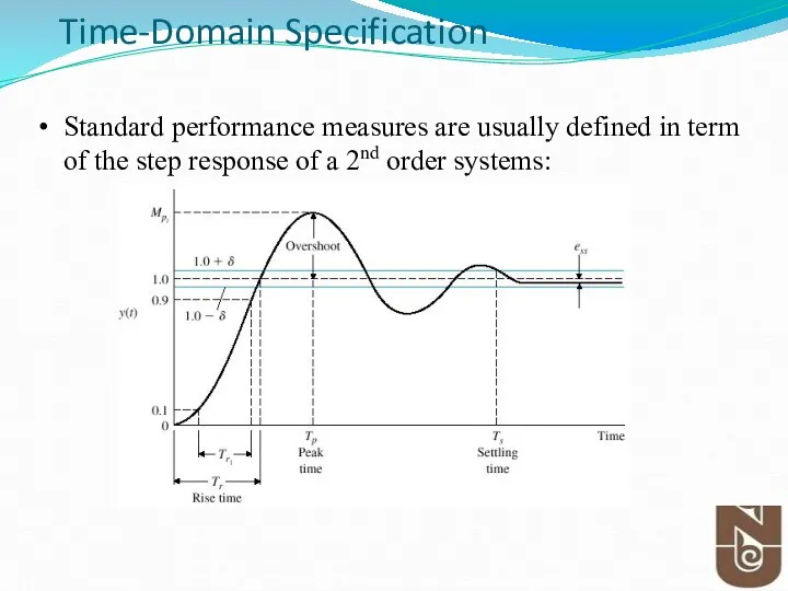
Time-Domain Specification
Standard performance measures are usually defined in term of the
Time-Domain Specification
Standard performance measures are usually defined in term of the
Time-Domain Specification
Standard performance measures are usually defined in term of the
Time-Domain Specification
Standard performance measures are usually defined in term of the
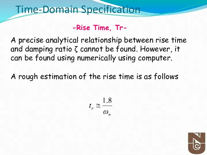
Time-Domain Specification
-Rise Time, Tr-
A precise analytical relationship between rise time and
Time-Domain Specification
-Rise Time, Tr-
A precise analytical relationship between rise time and
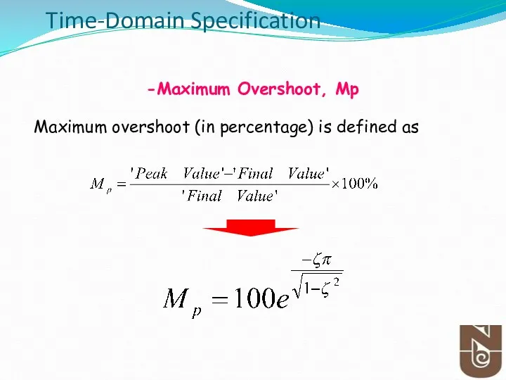
Time-Domain Specification
Maximum overshoot (in percentage) is defined as
-Maximum Overshoot, Mp
Time-Domain Specification
Maximum overshoot (in percentage) is defined as
-Maximum Overshoot, Mp
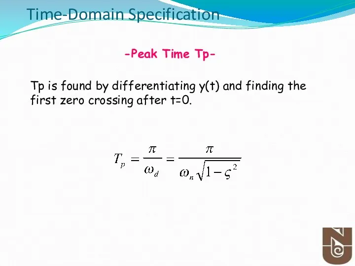
Time-Domain Specification
Tp is found by differentiating y(t) and finding the first
Time-Domain Specification
Tp is found by differentiating y(t) and finding the first
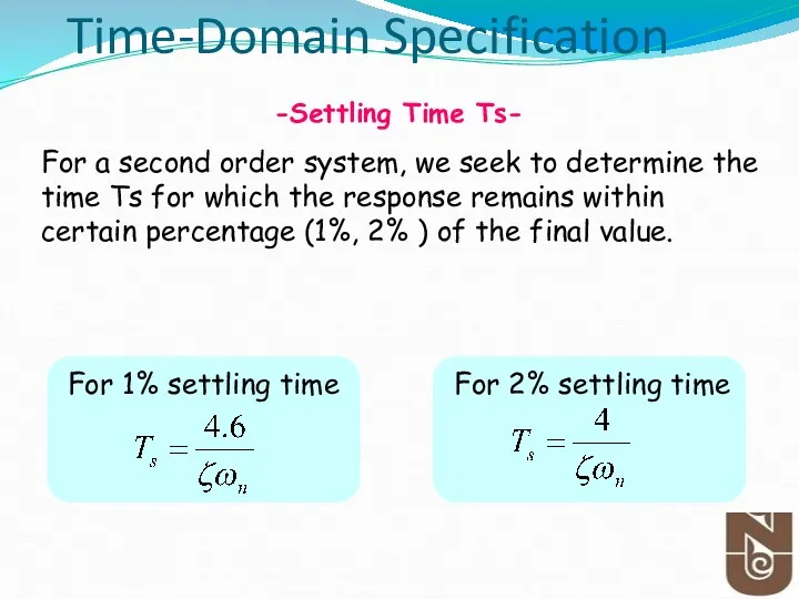
Time-Domain Specification
-Settling Time Ts-
For a second order system, we seek to
Time-Domain Specification
-Settling Time Ts-
For a second order system, we seek to
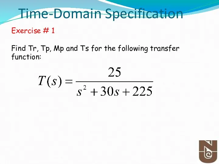
Time-Domain Specification
Exercise # 1
Find Tr, Tp, Mp and Ts for the
Time-Domain Specification
Exercise # 1
Find Tr, Tp, Mp and Ts for the

Time-Domain Specification
Exercise # 2
Find Tr, Tp, Mp and Ts for the
Time-Domain Specification
Exercise # 2
Find Tr, Tp, Mp and Ts for the
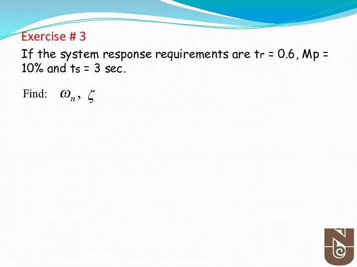
Exercise # 3
If the system response requirements are tr = 0.6,
Exercise # 3
If the system response requirements are tr = 0.6,
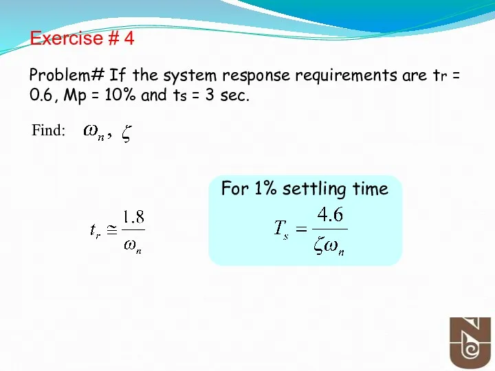
Exercise # 4
Problem# If the system response requirements are tr =
Exercise # 4
Problem# If the system response requirements are tr =
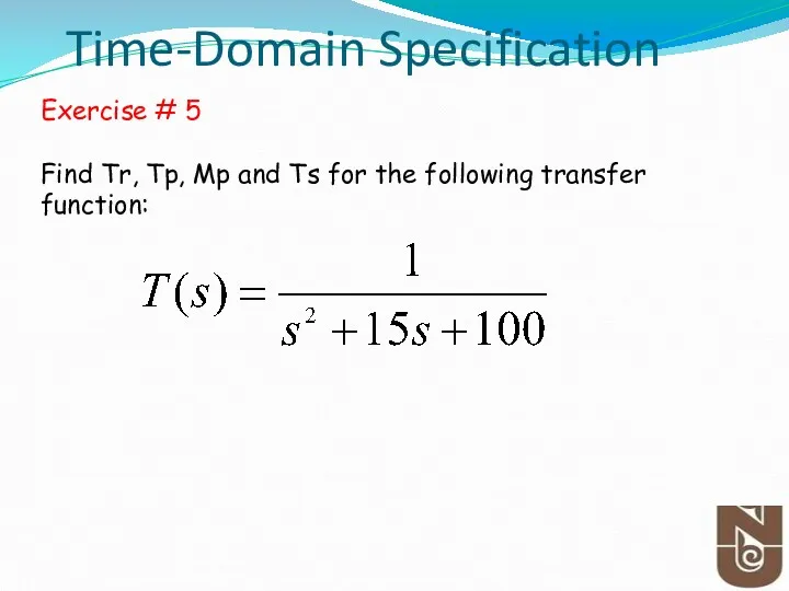
Time-Domain Specification
Exercise # 5
Find Tr, Tp, Mp and Ts for the
Time-Domain Specification
Exercise # 5
Find Tr, Tp, Mp and Ts for the

Time-Domain Specification
Exercise # 6
Find Tr, Tp, Mp and Ts for the
Time-Domain Specification
Exercise # 6
Find Tr, Tp, Mp and Ts for the

Time-Domain Specification
Exercise # 7
Find Tr, Tp, Mp and Ts for the
Time-Domain Specification
Exercise # 7
Find Tr, Tp, Mp and Ts for the
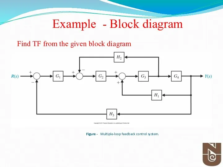
Figure - Multiple-loop feedback control system.
Example - Block diagram
Find TF
Figure - Multiple-loop feedback control system.
Example - Block diagram
Find TF
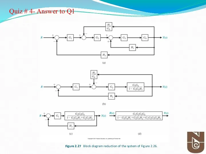
Figure 2.27 Block diagram reduction of the system of Figure 2.26.
Quiz
Figure 2.27 Block diagram reduction of the system of Figure 2.26.
Quiz
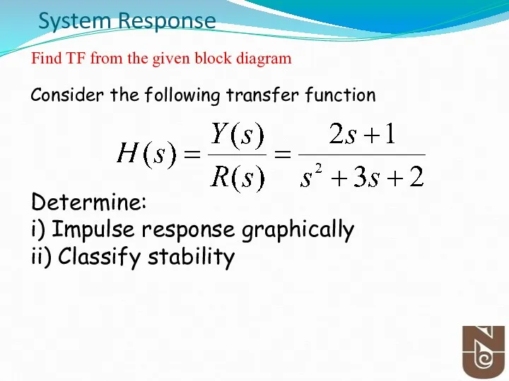
System Response
Consider the following transfer function
Determine:
i) Impulse response graphically
ii)
System Response
Consider the following transfer function
Determine:
i) Impulse response graphically
ii)
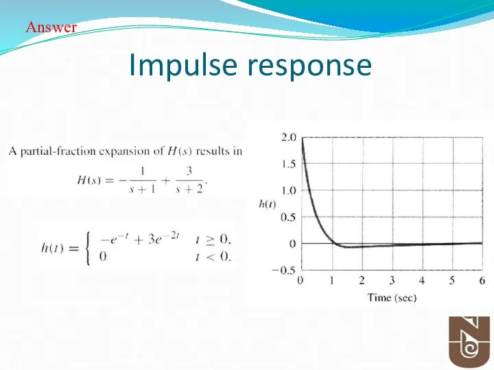
Impulse response
Answer
Impulse response
Answer

Midterm Exam
March 4, 2016, Friday, Time:8.00-9.00
Venue-6.141 & 5.103
Topics- Cover Until February
Midterm Exam
March 4, 2016, Friday, Time:8.00-9.00
Venue-6.141 & 5.103
Topics- Cover Until February

Tell me, I will forget!
Show me, I may remember!
Involve me, I
Tell me, I will forget! Show me, I may remember! Involve me, I
 Проводники с током в магнитном поле. Лекция 8
 Муфты приводов
 Магнитное поле в вакууме. (Лекция 7)
 Решение задач на дифракцию света
 Значение физики для объяснения мира и развития производительных сил общества
 Електричний струм в газах. Фізика. 8 клас
 Организация эксплуатации и ремонта бронетанковой техники. Ходовая часть
 Источники звука. Высота, тембр, громкость звука. Урок физики. 9 класс
 Сила трения. Автор Максимова Наталья Сергеевна
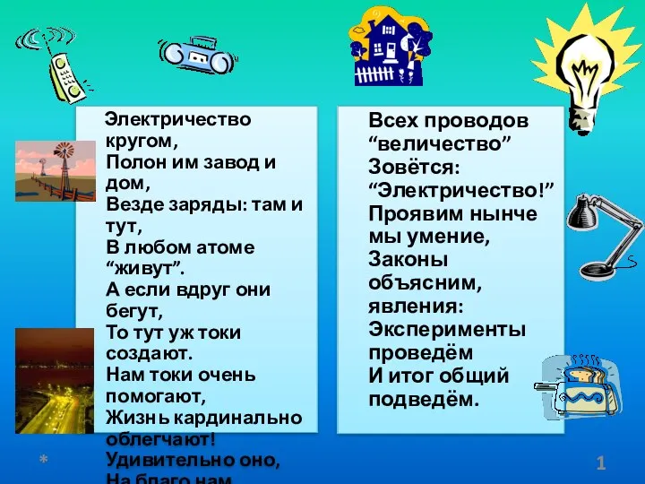 Электрические явления
 Загальна будова бойової машини піхоти БМП – 2, бронетранспортера БТР - 80
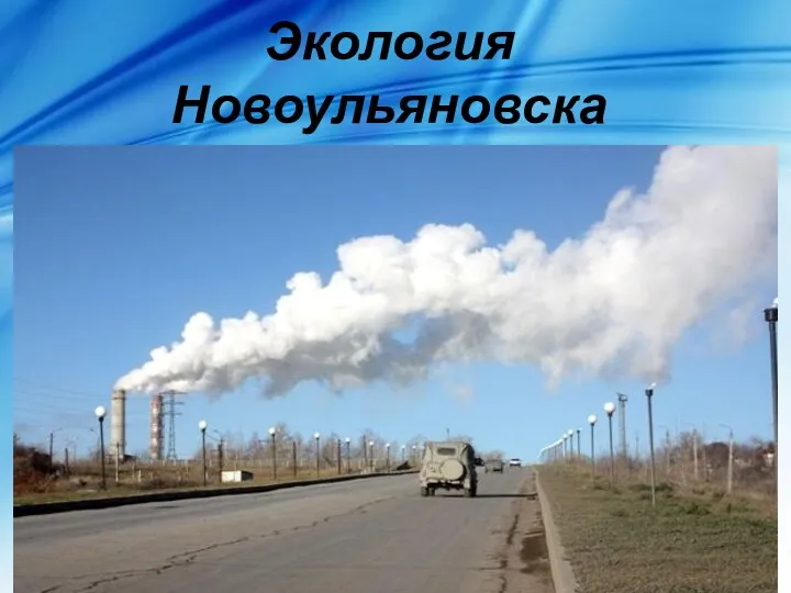 проект Экология города Новоульяновск
 Синтез нанокомпозитных материалов на основе субоксида кремния и наноструктур благородных металлов
 Сұйықтық және газ механикасы пәні
 Явление электромагнитной индукции
 Ремонт и обслуживание торгового оборудования
 Закат как физическое явление
 Машины переменного тока. Синхронные машины (СМ). Общие сведения. (Лекция 6)
 Подшипники качения
 Молекулярная физика и термодинамика
 Дисперсия света
 Техническое обслуживание электромеханических исполнительных механизмов
 Основы кинематики
 Цифровые ключи на биполярных транзисторах. Схемотехника, принципы работы, параметры и характеристики
 Регулирование напряжения в электрических сетях
 Электрическое и электромеханическое оборудование
 Тормоза и остановы. (Лекция № 3)
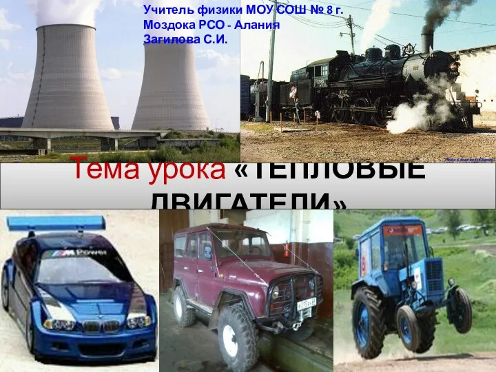 ТЕПЛОВЫЕ ДВИГАТЕЛИ