- Shunt and Series Compensation

Содержание
- 2. 2.1 Uniformly distributed fixed series and shunt compensation-1 The line performance is determined by the characteristic
- 3. 2.2 Uniformly distributed fixed series and shunt compensation-2 With shunt compensation: Degree of shunt compensation: Characteristic
- 4. 2.3 Uniformly distributed fixed series and shunt compensation-3 With series compensation: Degree of series compensation: Characteristic
- 5. 2.4 Uniformly distributed fixed series and shunt compensation-4 With both series and shunt compensation: Line angle
- 6. 2.5 The effect of compensation on voltage-1 Light load inductive shunt compensation; with ksh = 1
- 7. 2.6 The effect of compensation on voltage-1 Light load inductive shunt compensation; with ksh = 1
- 8. 2.7 The effect of compensation on voltage-2 series capacitive compensation may be used instead of shunt
- 9. 2.8 The effect of compensation on voltage-2 series capacitive compensation may be used instead of shunt
- 10. 2.9 The effect on maximum power How to increase maximum power? Decrease Zc’; Decrease θ’; Decrease
- 11. 2.10 Uniformly distributed regulated shunt compensation For the 600 km, 500 kV line:
- 12. 2.11 Regulated compensation at discrete intervals
- 13. 2.12 Performance of a 600 km line with an SVS regulating midpoint voltage
- 14. 2.13 Arbitrary number of regulated compensators
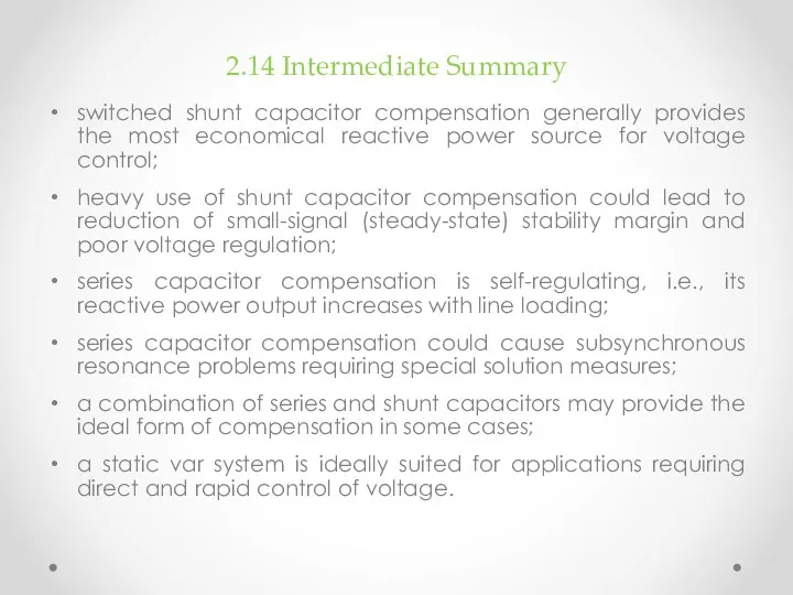
- 15. 2.14 Intermediate Summary switched shunt capacitor compensation generally provides the most economical reactive power source for
- 16. Series Capacitors
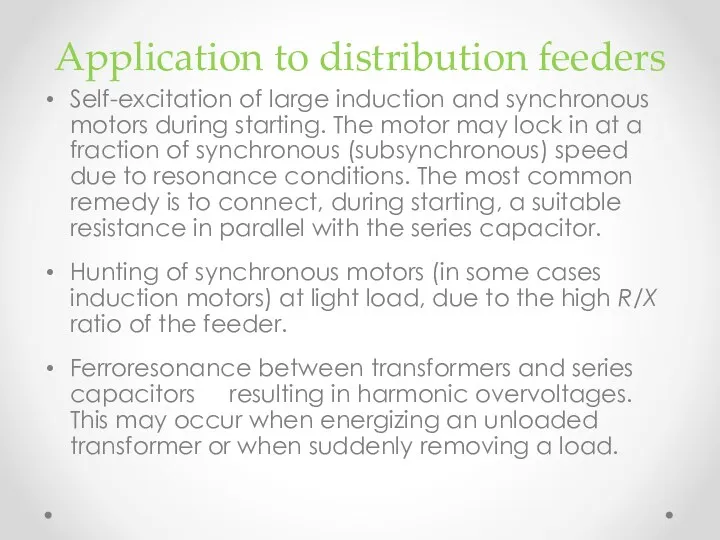
- 17. Application to distribution feeders Self-excitation of large induction and synchronous motors during starting. The motor may
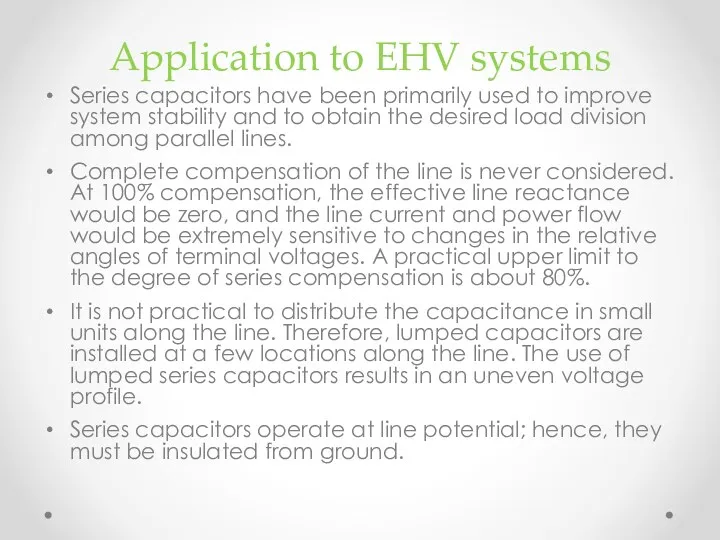
- 18. Application to EHV systems Series capacitors have been primarily used to improve system stability and to
- 19. Voltage rise due to reactive current Voltage rise on one side of the capacitor may be
- 20. Bypassing and reinsertion The series capacitors are normally subjected to a voltage which is on the
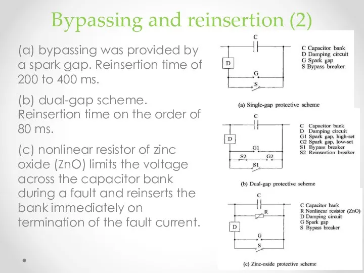
- 21. Bypassing and reinsertion (2) (a) bypassing was provided by a spark gap. Reinsertion time of 200
- 22. Location of SC A series-capacitor bank can theoretically be located anywhere along the line. Factors influencing
- 23. GTO Thyristor-Controlled Series Capacitor (GCSC)
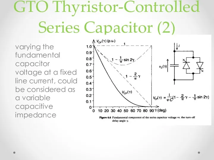
- 24. GTO Thyristor-Controlled Series Capacitor (2) varying the fundamental capacitor voltage at a fixed line current, could
- 25. Thyristor-Switched Series Capacitor (TSSC)
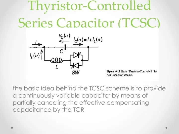
- 26. Thyristor-Controlled Series Capacitor (TCSC) the basic idea behind the TCSC scheme is to provide a continuously
- 27. Impedance-delay angle characteristic of TCSC
- 28. Shunt compensation. Static VAR systems
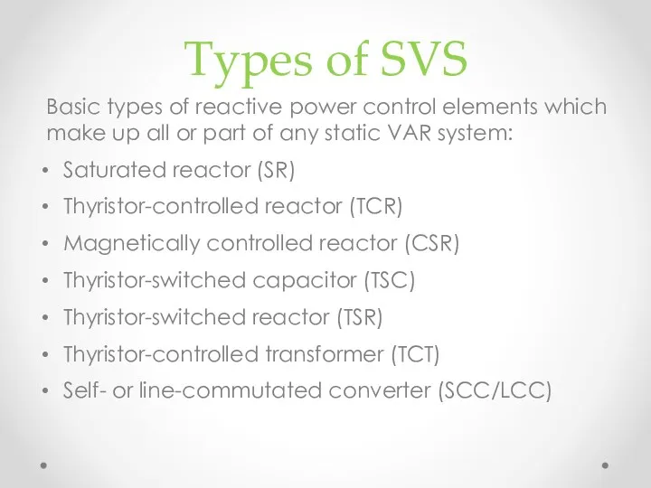
- 29. Types of SVS Basic types of reactive power control elements which make up all or part
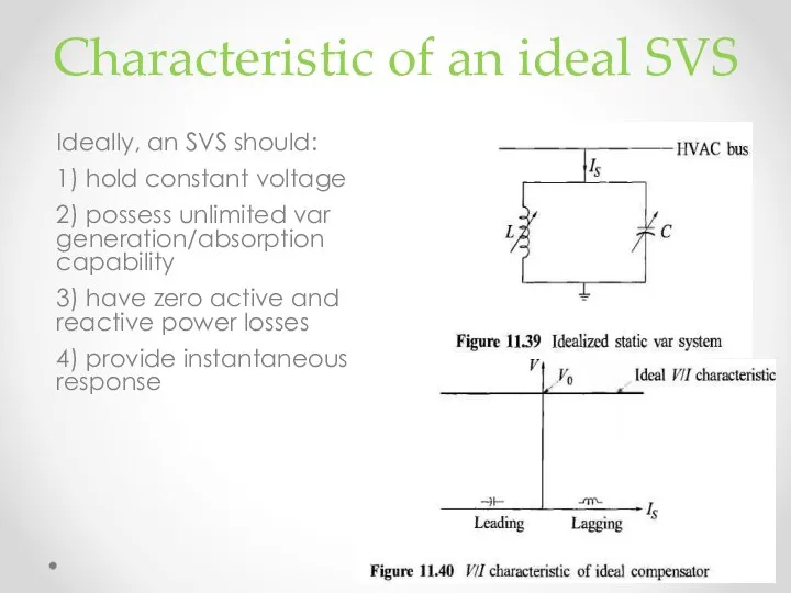
- 30. Characteristic of an ideal SVS Ideally, an SVS should: 1) hold constant voltage 2) possess unlimited
- 31. Composite characteristics of SVS
- 32. Power system characteristic The Thevenin impedance is predominantly an inductive reactance. The voltage V increases linearly
- 33. Composite SVS - power system characteristic Graphically illustrated solution of SVS and power system characteristic equations.
- 34. The effect of switched capacitors
- 35. Thyristor-controlled reactor (TCR) Generates harmonics
- 36. Thyristor-switched capacitor (TSC) The thyristor firing controls are designed to minimize the switching transients
- 37. Practical SVC Applications : Control of temporary overvoltages Prevention of voltage collapse Enhancement of transient stability
- 38. VSC-based compensators VSC-based compensators construction
- 39. Insulated Gate Bipolar Transistors (IGBT) vs Power Thyristors Thyristors can only be turned on (not off)
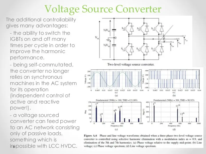
- 40. Voltage Source Converter The additional controllability gives many advantages: - the ability to switch the IGBTs
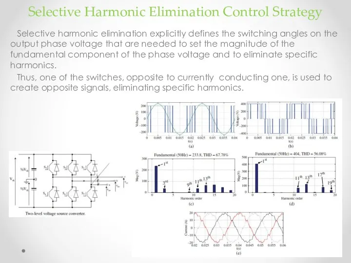
- 41. Selective Harmonic Elimination Control Strategy Selective harmonic elimination explicitly defines the switching angles on the output
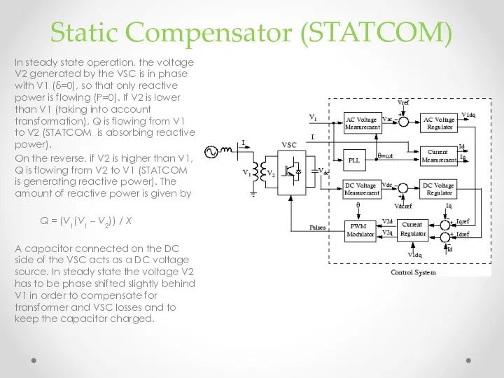
- 42. Static Compensator (STATCOM) In steady state operation, the voltage V2 generated by the VSC is in
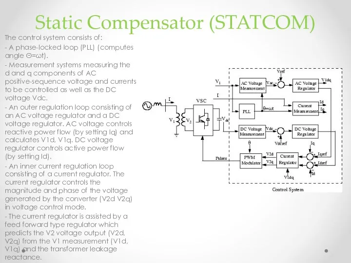
- 43. Static Compensator (STATCOM) The control system consists of: - A phase-locked loop (PLL) (computes angle Θ=ωt).
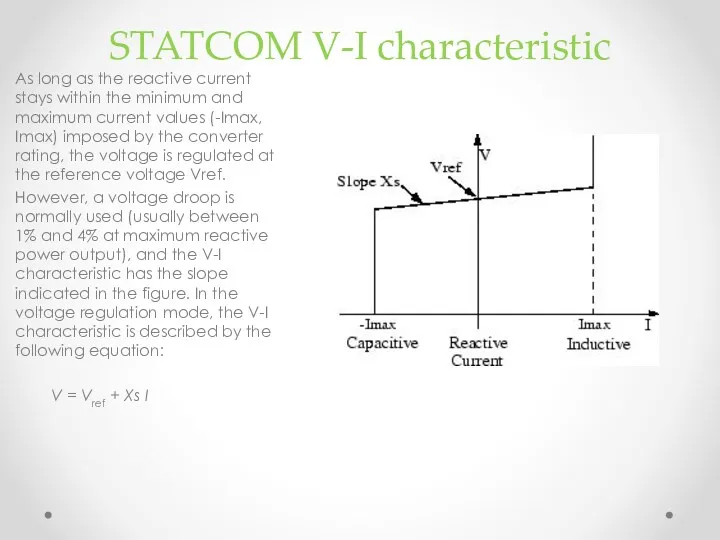
- 44. STATCOM V-I characteristic As long as the reactive current stays within the minimum and maximum current
- 45. STATCOM Grid Operation
- 46. STATCOM Grid Operation
- 47. STATCOM Application for Wind Farms – Typical Installation
- 48. STATCOM Application for Wind Farms - LVRT
- 49. STATCOM Application for Wind Farms – Transient Response
- 50. STATCOM vs SVC
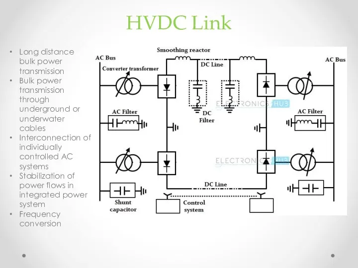
- 51. HVDC Link Long distance bulk power transmission Bulk power transmission through underground or underwater cables Interconnection
- 52. HVDC Link Advantages In DC transmission, only two conductors are needed for a single line. It
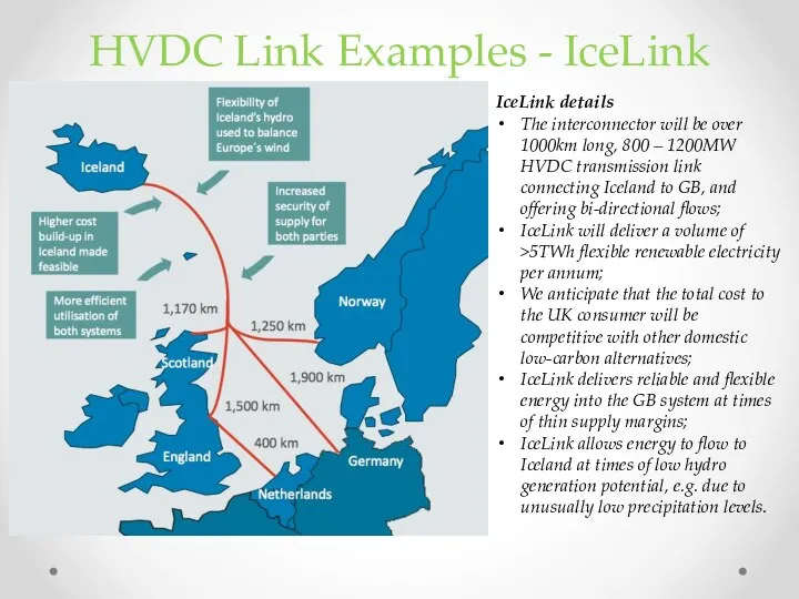
- 53. HVDC Link Examples - IceLink IceLink details The interconnector will be over 1000km long, 800 –
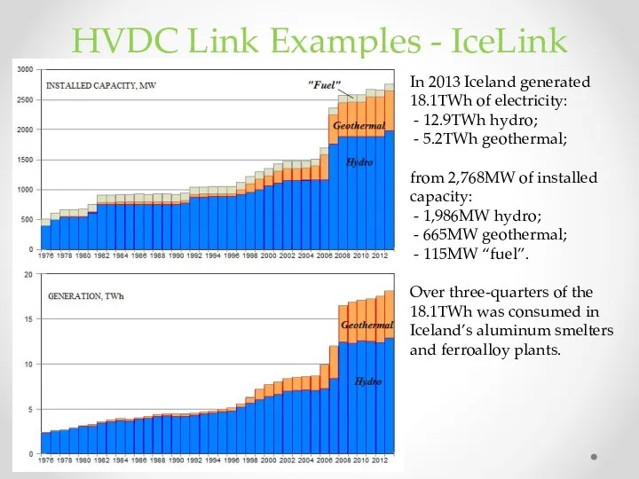
- 54. HVDC Link Examples - IceLink In 2013 Iceland generated 18.1TWh of electricity: - 12.9TWh hydro; -
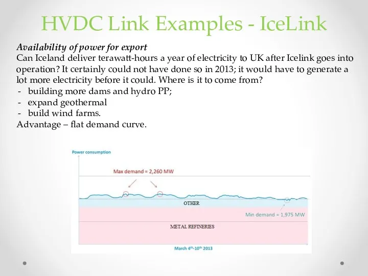
- 55. HVDC Link Examples - IceLink Availability of power for export Can Iceland deliver terawatt-hours a year
- 56. HVDC Link Examples - IceLink Power imports from Iceland IceLink will have a capacity of only
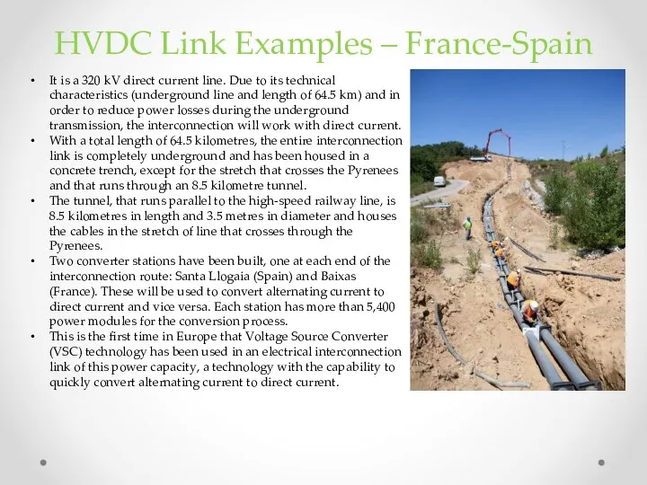
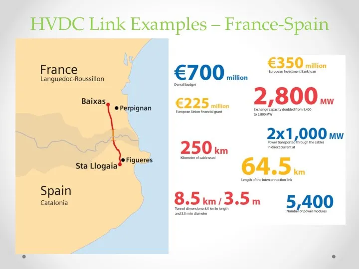
- 57. HVDC Link Examples – France-Spain It is a 320 kV direct current line. Due to its
- 58. HVDC Link Examples – France-Spain
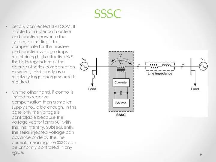
- 59. SSSC Serially connected STATCOM. It is able to transfer both active and reactive power to the
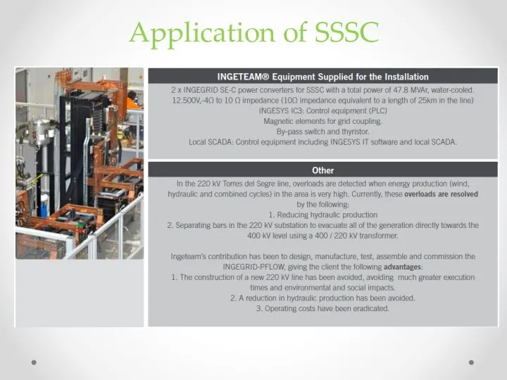
- 60. Application of SSSC
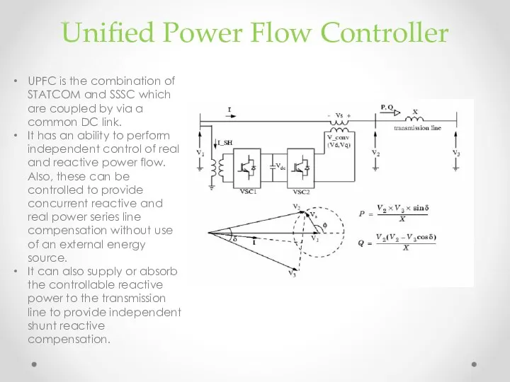
- 61. Unified Power Flow Controller UPFC is the combination of STATCOM and SSSC which are coupled by
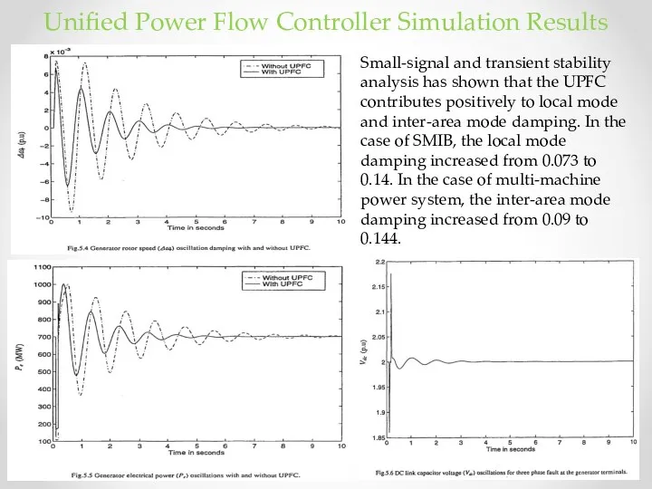
- 62. Unified Power Flow Controller Simulation Results Small-signal and transient stability analysis has shown that the UPFC
- 64. Скачать презентацию
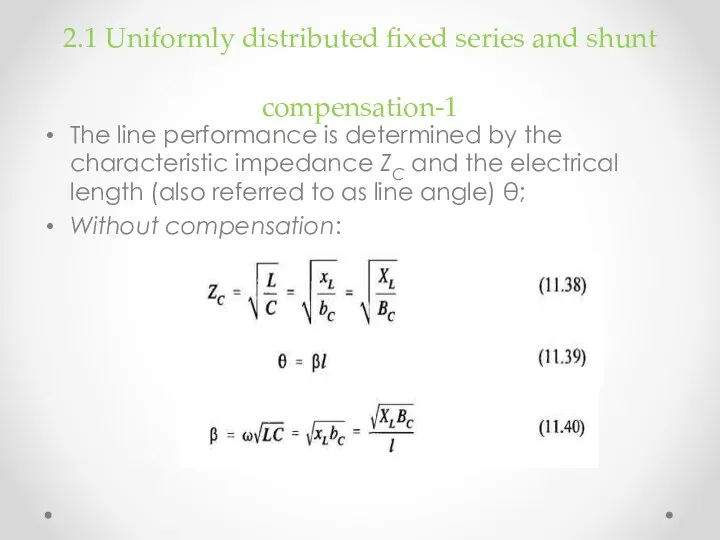
2.1 Uniformly distributed fixed series and shunt compensation-1
The line performance is
2.1 Uniformly distributed fixed series and shunt compensation-1
The line performance is
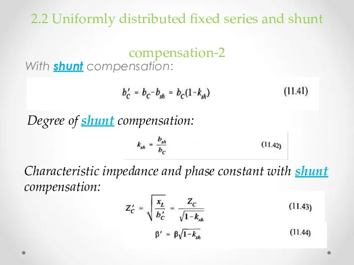
2.2 Uniformly distributed fixed series and shunt compensation-2
With shunt compensation:
Degree of
2.2 Uniformly distributed fixed series and shunt compensation-2
With shunt compensation:
Degree of
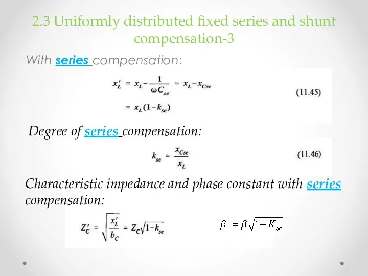
2.3 Uniformly distributed fixed series and shunt compensation-3
With series compensation:
Degree of
2.3 Uniformly distributed fixed series and shunt compensation-3
With series compensation:
Degree of
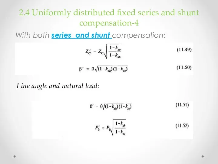
2.4 Uniformly distributed fixed series and shunt compensation-4
With both series and
2.4 Uniformly distributed fixed series and shunt compensation-4
With both series and
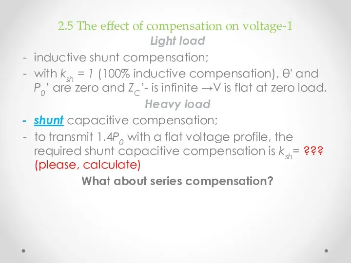
2.5 The effect of compensation on voltage-1
Light load
inductive shunt compensation;
with ksh
2.5 The effect of compensation on voltage-1
Light load
inductive shunt compensation;
with ksh
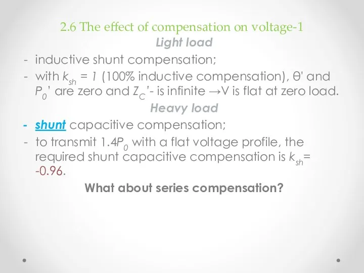
2.6 The effect of compensation on voltage-1
Light load
inductive shunt compensation;
with ksh
2.6 The effect of compensation on voltage-1
Light load
inductive shunt compensation;
with ksh

2.7 The effect of compensation on voltage-2
series capacitive compensation may be
2.7 The effect of compensation on voltage-2
series capacitive compensation may be
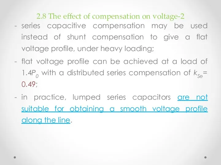
2.8 The effect of compensation on voltage-2
series capacitive compensation may be
2.8 The effect of compensation on voltage-2
series capacitive compensation may be
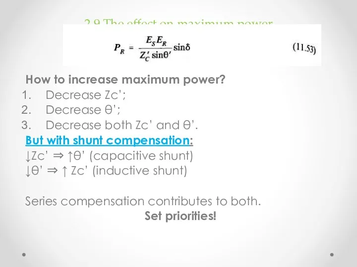
2.9 The effect on maximum power
How to increase maximum power?
Decrease Zc’;
Decrease
2.9 The effect on maximum power
How to increase maximum power?
Decrease Zc’;
Decrease
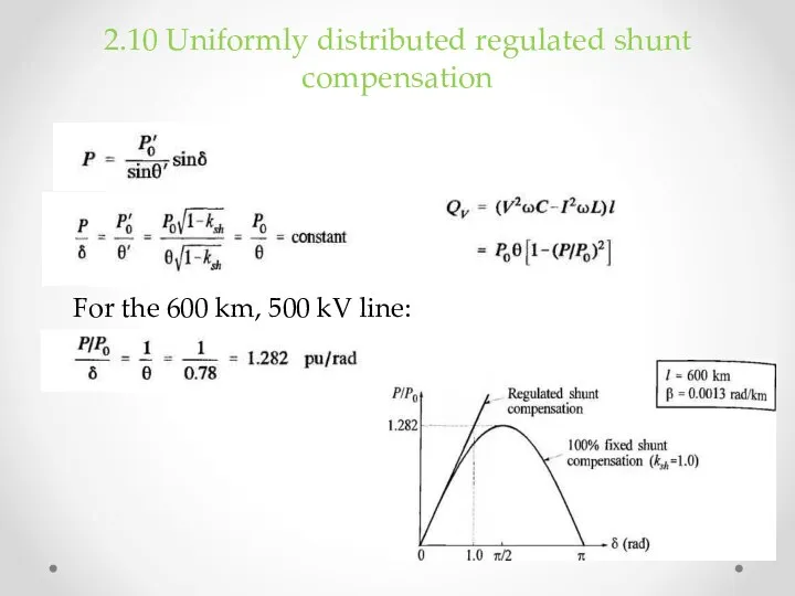
2.10 Uniformly distributed regulated shunt compensation
For the 600 km, 500 kV
2.10 Uniformly distributed regulated shunt compensation
For the 600 km, 500 kV
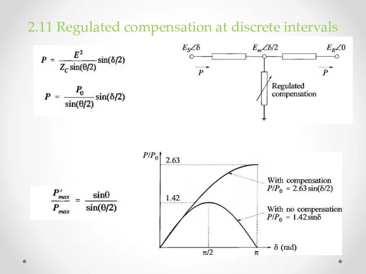
2.11 Regulated compensation at discrete intervals
2.11 Regulated compensation at discrete intervals
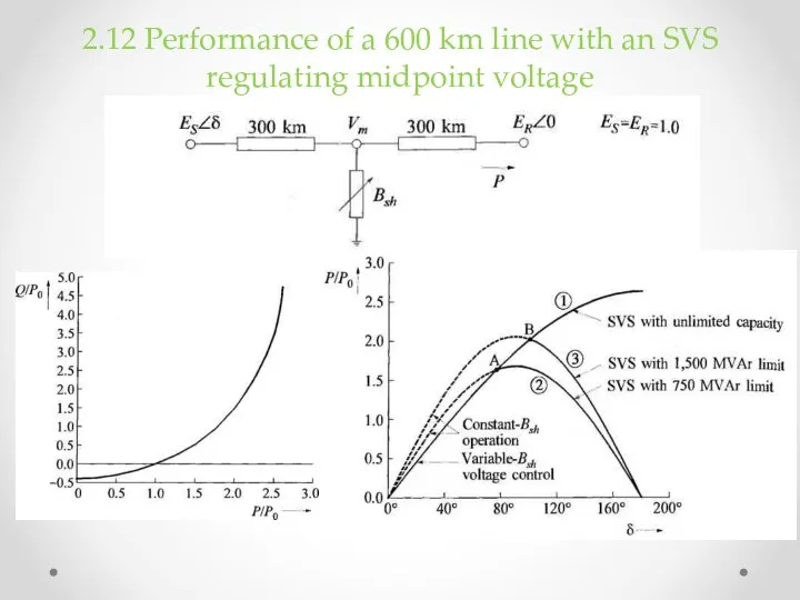
2.12 Performance of a 600 km line with an SVS regulating
2.12 Performance of a 600 km line with an SVS regulating
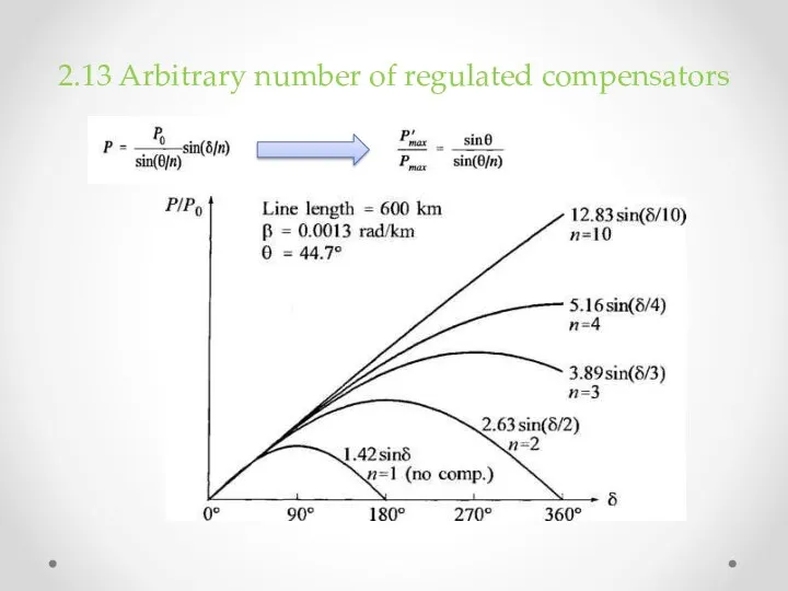
2.13 Arbitrary number of regulated compensators
2.13 Arbitrary number of regulated compensators
2.14 Intermediate Summary
switched shunt capacitor compensation generally provides the most economical
2.14 Intermediate Summary
switched shunt capacitor compensation generally provides the most economical
Series Capacitors
Series Capacitors
Application to distribution feeders
Self-excitation of large induction and synchronous motors during
Application to distribution feeders
Self-excitation of large induction and synchronous motors during
Application to EHV systems
Series capacitors have been primarily used to improve
Application to EHV systems
Series capacitors have been primarily used to improve
Voltage rise due to reactive current
Voltage rise on one side of
Voltage rise due to reactive current
Voltage rise on one side of
Bypassing and reinsertion
The series capacitors are normally subjected to a voltage
Bypassing and reinsertion
The series capacitors are normally subjected to a voltage
Bypassing and reinsertion (2)
(a) bypassing was provided by a spark gap.
Bypassing and reinsertion (2)
(a) bypassing was provided by a spark gap.
Location of SC
A series-capacitor bank can theoretically be located anywhere along
Location of SC
A series-capacitor bank can theoretically be located anywhere along
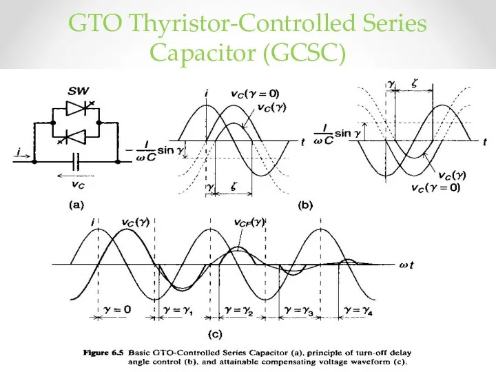
GTO Thyristor-Controlled Series Capacitor (GCSC)
GTO Thyristor-Controlled Series Capacitor (GCSC)
GTO Thyristor-Controlled Series Capacitor (2)
varying the fundamental capacitor voltage at a
GTO Thyristor-Controlled Series Capacitor (2)
varying the fundamental capacitor voltage at a
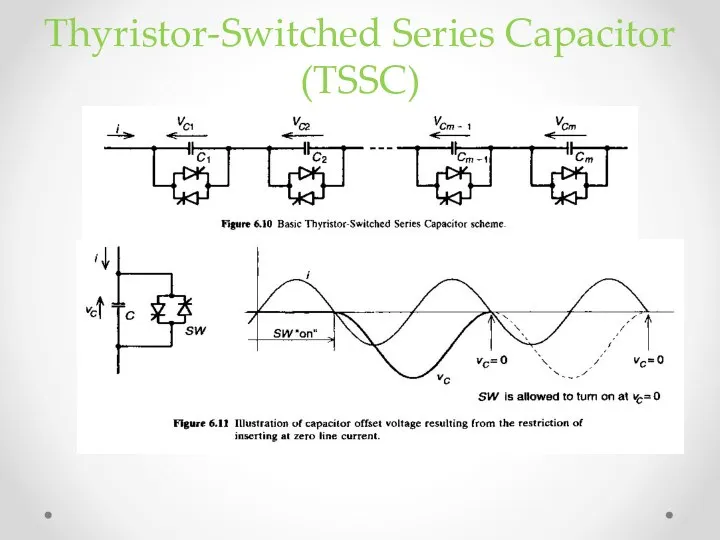
Thyristor-Switched Series Capacitor (TSSC)
Thyristor-Switched Series Capacitor (TSSC)
Thyristor-Controlled Series Capacitor (TCSC)
the basic idea behind the TCSC scheme is
Thyristor-Controlled Series Capacitor (TCSC)
the basic idea behind the TCSC scheme is
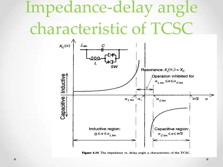
Impedance-delay angle characteristic of TCSC
Impedance-delay angle characteristic of TCSC
Shunt compensation. Static VAR systems
Shunt compensation. Static VAR systems
Types of SVS
Basic types of reactive power control elements which make
Types of SVS
Basic types of reactive power control elements which make
Characteristic of an ideal SVS
Ideally, an SVS should:
1) hold constant voltage
2)
Characteristic of an ideal SVS
Ideally, an SVS should:
1) hold constant voltage
2)
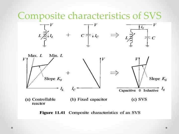
Composite characteristics of SVS
Composite characteristics of SVS
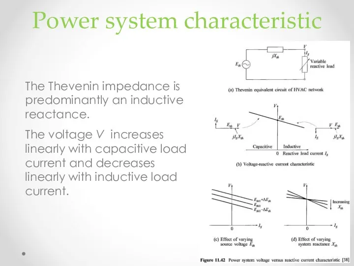
Power system characteristic
The Thevenin impedance is predominantly an inductive reactance.
The
Power system characteristic
The Thevenin impedance is predominantly an inductive reactance.
The
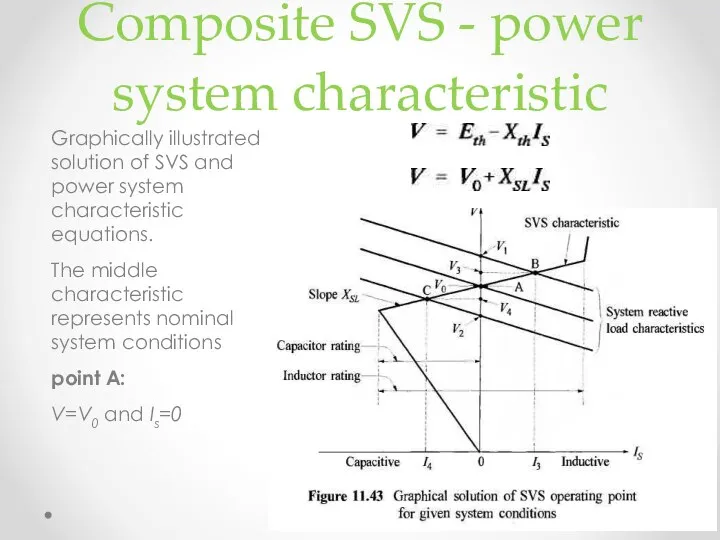
Composite SVS - power system characteristic
Graphically illustrated solution of SVS and
Composite SVS - power system characteristic
Graphically illustrated solution of SVS and
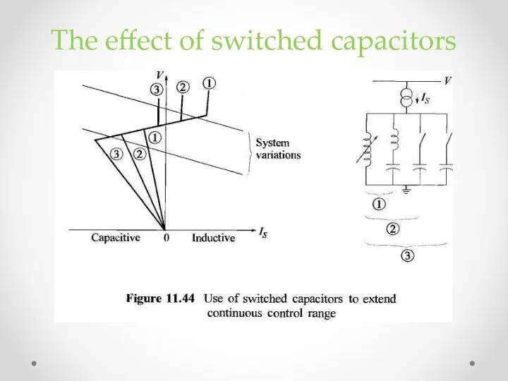
The effect of switched capacitors
The effect of switched capacitors
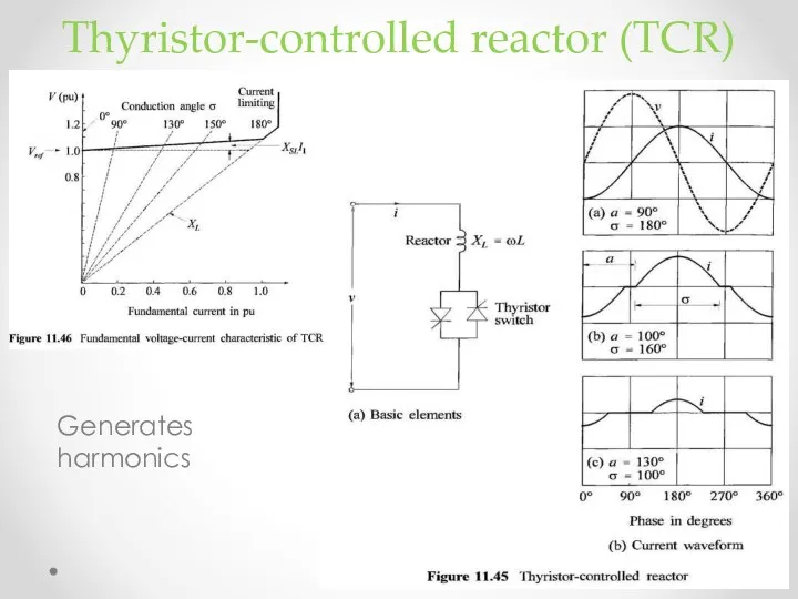
Thyristor-controlled reactor (TCR)
Generates harmonics
Thyristor-controlled reactor (TCR)
Generates harmonics
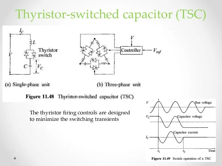
Thyristor-switched capacitor (TSC)
The thyristor firing controls are designed to minimize the
Thyristor-switched capacitor (TSC)
The thyristor firing controls are designed to minimize the
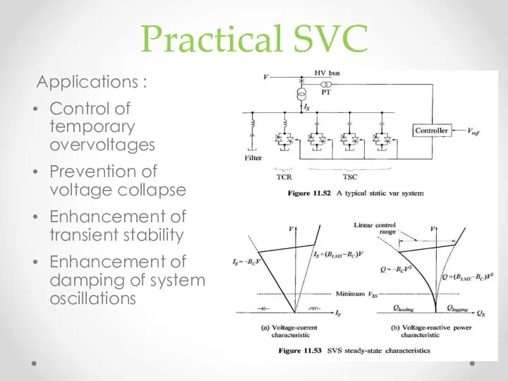
Practical SVC
Applications :
Control of temporary overvoltages
Prevention of voltage collapse
Enhancement of transient
Practical SVC
Applications :
Control of temporary overvoltages
Prevention of voltage collapse
Enhancement of transient
VSC-based compensators
VSC-based compensators construction
VSC-based compensators
VSC-based compensators construction
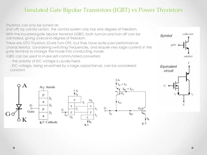
Insulated Gate Bipolar Transistors (IGBT) vs Power Thyristors
Thyristors can only be
Insulated Gate Bipolar Transistors (IGBT) vs Power Thyristors
Thyristors can only be
Voltage Source Converter
The additional controllability gives many advantages:
- the ability
Voltage Source Converter
The additional controllability gives many advantages:
- the ability
Selective Harmonic Elimination Control Strategy
Selective harmonic elimination explicitly defines the switching
Selective Harmonic Elimination Control Strategy
Selective harmonic elimination explicitly defines the switching
Static Compensator (STATCOM)
In steady state operation, the voltage V2 generated by
Static Compensator (STATCOM)
In steady state operation, the voltage V2 generated by
Static Compensator (STATCOM)
The control system consists of:
- A phase-locked loop (PLL)
Static Compensator (STATCOM)
The control system consists of:
- A phase-locked loop (PLL)
STATCOM V-I characteristic
As long as the reactive current stays within the
STATCOM V-I characteristic
As long as the reactive current stays within the
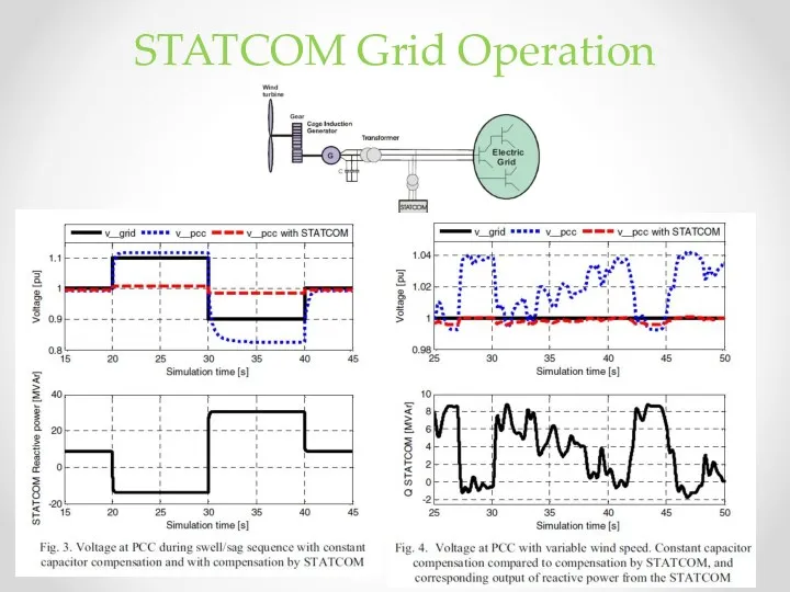
STATCOM Grid Operation
STATCOM Grid Operation
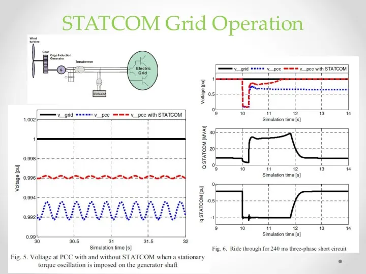
STATCOM Grid Operation
STATCOM Grid Operation
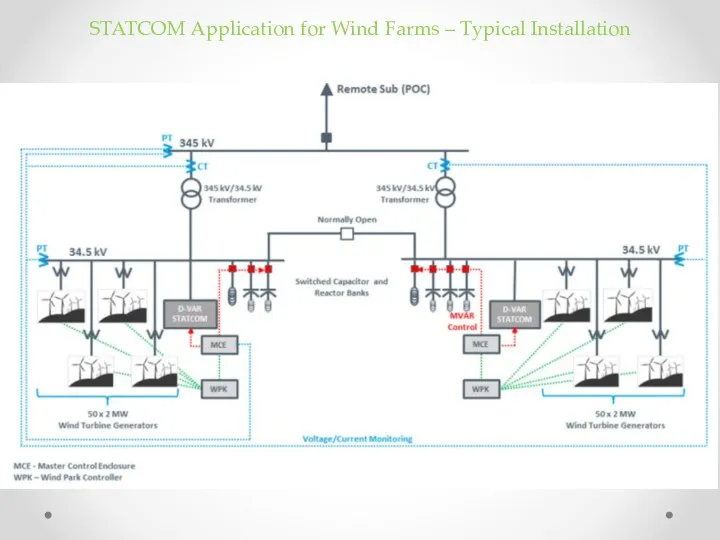
STATCOM Application for Wind Farms – Typical Installation
STATCOM Application for Wind Farms – Typical Installation
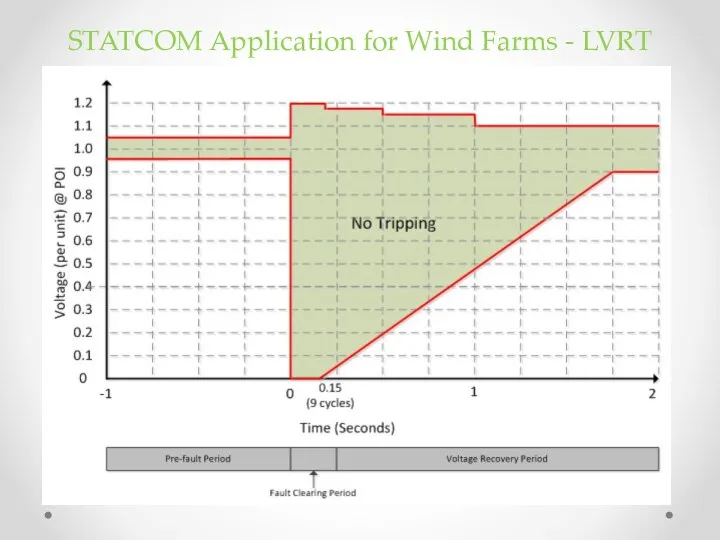
STATCOM Application for Wind Farms - LVRT
STATCOM Application for Wind Farms - LVRT
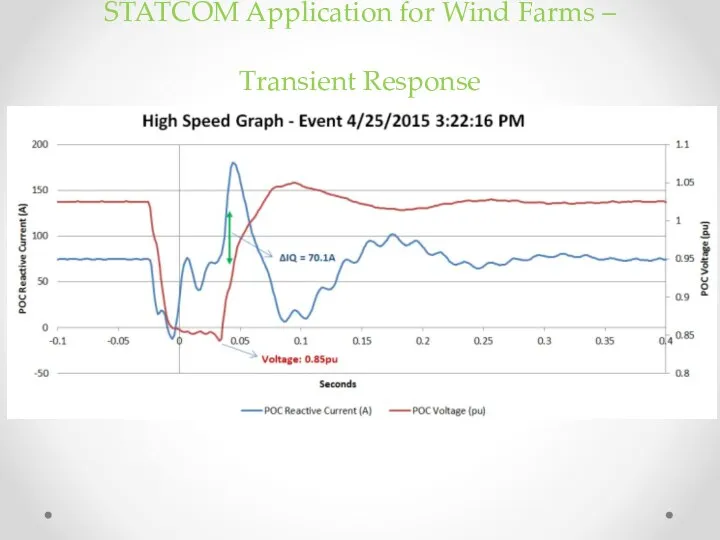
STATCOM Application for Wind Farms – Transient Response
STATCOM Application for Wind Farms – Transient Response
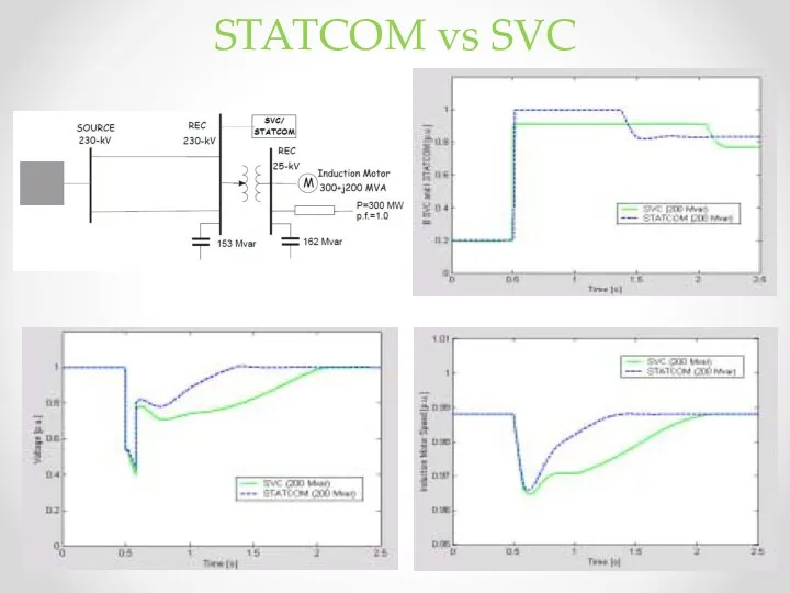
STATCOM vs SVC
STATCOM vs SVC
HVDC Link
Long distance bulk power transmission
Bulk power transmission through underground or
HVDC Link
Long distance bulk power transmission
Bulk power transmission through underground or
HVDC Link Advantages
In DC transmission, only two conductors are needed for
HVDC Link Advantages
In DC transmission, only two conductors are needed for
HVDC Link Examples - IceLink
IceLink details
The interconnector will be over 1000km
HVDC Link Examples - IceLink
IceLink details
The interconnector will be over 1000km
HVDC Link Examples - IceLink
In 2013 Iceland generated 18.1TWh of electricity:
HVDC Link Examples - IceLink
In 2013 Iceland generated 18.1TWh of electricity:
HVDC Link Examples - IceLink
Availability of power for export
Can Iceland deliver
HVDC Link Examples - IceLink
Availability of power for export
Can Iceland deliver
HVDC Link Examples - IceLink
Power imports from Iceland
IceLink will have a
HVDC Link Examples - IceLink
Power imports from Iceland
IceLink will have a
HVDC Link Examples – France-Spain
It is a 320 kV direct current
HVDC Link Examples – France-Spain
It is a 320 kV direct current
HVDC Link Examples – France-Spain
HVDC Link Examples – France-Spain
SSSC
Serially connected STATCOM. It is able to transfer both active and
SSSC
Serially connected STATCOM. It is able to transfer both active and
Application of SSSC
Application of SSSC
Unified Power Flow Controller
UPFC is the combination of STATCOM and SSSC
Unified Power Flow Controller
UPFC is the combination of STATCOM and SSSC
Unified Power Flow Controller Simulation Results
Small-signal and transient stability analysis has
Unified Power Flow Controller Simulation Results
Small-signal and transient stability analysis has
 Затухающие и вынужденные колебания. Уравнение затухающих колебаний
 Классификация веществ по проводимости
 Основные характеристики звеньев и систем. Временные характеристики
 Обучение физике на основе индивидуального и дифференцированного подхода
 Оптические приборы
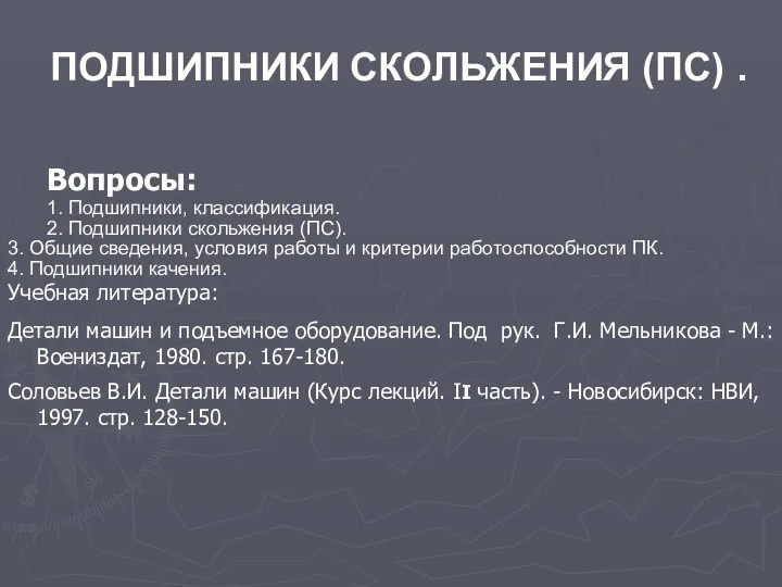 Подшипники скольжения (ПС)
 Точність обробки. (Лекция 3)
 Русские изобретения, без которых нельзя представить современный мир
 Реактивное движение
 Технологический процесс изготовления детали Шестерня
 Подъемно-поворотные сварочные колонны
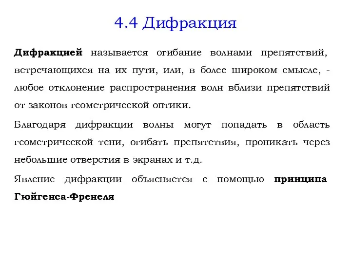 Дифракция. Принцип Гюйгенса-Френеля
 SCR - Система каталитического восстановления выхлопных газов на двигателях Weichai Euro 4 & 5
 Презентация МАРИЯ СКЛОДОВСКАЯ-КЮРИ
 Теория космических полётов
 Тема 3. Фізичні властивості гірських порід
 Экспериментальные методы исследования частиц
 Презентация Основные положения МКТ (10 класс)
 Гамма-излучение
 Физические свойства воды
 Условия плавания тел в жидкости. Лабораторная работа
 ИСО и примеры сил
 Тема 8. Методы автоматического регулирования параметров технологических систем. Лекция 23
 Архимедова сила
 Предмет радиотеоэкологии. Цель и задачи радиотеоэкологии
 Презентация:Каты җисемнәрдә, сыеклыкларда һәм газларда басым.
 КДР подготовка
 Силы в природе