- Association analysis

Содержание
- 2. Naive algorithm (1) Given a set of items I and a database D Generate all possible
- 3. Naive algorithm (2) Consider the dataset D from the previous example: A set of items I
- 4. Naive algorithm (3) How can we restrict a number of generated association rules to avoid the
- 5. Naive algorithm (4) If the support of the set (X, Y) is less than minsup, then
- 6. General algorithm of association rule discovery Algorithm 1.1: General algorithm of association rule discovery Find all
- 7. Rule Generation Algorithm Algorithm 1.2: Rule generation. for each frequent itemset Li do for each subset
- 8. Algorithm 1.3: Apriori Notation: Assume that all transactions are internally ordered Lk denotes a set of
- 9. Algorithm 1.3: Apriori str.
- 10. Function: Apriori_Gen(Ck) (1) Algoritm 1.3: Frequent itemsets discovery algorithm (Apriori) In: frequent (k-1)-itemsets Lk-1 Out: candidate
- 11. Function: Apriori_Gen(Ck) (2) Algorytm 1.3: Frequent itemsets discovery algorithm (Apriori) In: frequent (k-1)-itemsets Lk-1 Out: candidate
- 12. Example 2 Assume that minsup = 50% (2 transactions) C1 L1
- 13. Example 2 (cont.) C2 L2 C3 L3 C4 = ∅ L4 = ∅
- 14. Apriori Candidate Generation (1) Given Lk, generate Ck+1 in two steps: 1. Join step: Join Lk1
- 15. Apriori Candidate Generation (2) Given L2 L2 C3 – after join join prune C3 – final
- 16. {} A B C D AB AC AD BC BD CD ABC ABD ACD BCD ABCD
- 17. Properties of measures Monotonicity property Let I be a set of items, and J = 2|I|
- 18. Why does it work? (1) Anti-monotone property of the support measure: all subsets of a frequent
- 19. Apriori Property ∅ A B C D AB AC AD BC BD CD ABC ABD ACD
- 20. Why does it work? (2) The join step is equivalent to extending each itemset in Lk
- 21. Discovering Rules L3 23 → 5 support = 2 confidence = 100% 25 → 3 support
- 22. Rule generation (1) For each k-itemset X we can produce up to 2k – 2 association
- 23. Rule generation (2) Given a frequent iteset Y Theorem: if a rule X → Y –
- 24. Rule generation (3) a, b, c, d → {} b, c, d → a a, c,
- 25. Example 2 Given the following database: Assume the following values for minsup and minconf: minsup =
- 26. Example 2 (cont.) C1 L1 C2 L2
- 27. Example 2 (cont.) C3 L3 C4 = ∅ L4 = ∅ This is the end of
- 28. Example 2 (cont.) rule generation fi sup rule conf 1 0.40 beer → sugar 0.67 1
- 29. Example 2 (cont.) rule generation fi sup rule conf 1 0.40 sugar → beer 1.00 2
- 30. Closed frequent itemsets (1) In any large dataset we can discover millions of frequent itemsets which
- 31. Closed frequent itemsets (2) An itemset X is a closed in the dataset D if none
- 32. Closed frequent itemsets (3) From a set of closed frequent itemsets we can derive all frequent
- 33. Closed frequent itemsets (4) str. dataset Assume that the minimum support threshold minsup = 30% (2
- 34. Semi-lattice of closed itemsets str. {} A B C D AB AC AD BC BD CD
- 35. Semi-lattice of frequent itemsets str. A B C D AB AC AD BC BD CD ABC
- 36. Semi-lattice of closed frequent itemsets str. {} A B C D AB AC AD BC BD
- 37. Generation of frequent itemsets from a set of closed frequent itemsets (1) Let FI denotes a
- 38. Generation of frequent itemsets from a set of closed frequent itemsets (2) for i= 1 to
- 39. Generation of frequent itemsets from a set of closed frequent itemsets (3) Example: FI = ∅;
- 40. Generation of frequent itemsets from a set of closed frequent itemsets (4) Example (cd.): Subset (B,
- 41. Maximal frequent itemsets (1) An itemset X is a maximal frequent itemset in the dataset D
- 42. Maximal frequent itemsets (2) Let us consider the dataset given below: str.
- 43. Maximal frequent itemsets (3) str. {} A B C D AB AC AD BC BD CD
- 44. Maximal frequent itemsets (4) Maximal frequent itemsets: (A, B) and (B, C, D) Easy to notice
- 45. Generalized Association Rules or Multilevel Association Rules
- 46. Multilevel AR (1) It is difficult to find interesting, strong associations among data items at a
- 47. Multilevel AR (2) Multilevel association rule: „50% of clients who purchase bread-stuff (bread, rolls, croissants, etc.)
- 48. Multilevel AR - item hierarchy An attribute (item) may be generalized or specialized according to a
- 49. Item hierarchy Item hierarchy (dimension hierarchy) – semantic classification of items It describes generalization/specialization relationship among
- 50. Basic algorithm (1) Extend each transaction Ti ∈ D by adding all ancestors of each item
- 51. Basic algorithm (2) A trivial multilevel association rule is the rule of the form „node →
- 52. Drawbacks of the basic algorithm Drawbacks of the approach: The number of candidate itemsets is much
- 53. MAR: uniform support vs. reduced support Uniform support: the same minimum support for all levels one
- 54. MAR: uniform support vs. reduced support Reduced Support: reduced minimum support at lower levels - different
- 56. Скачать презентацию
 Программное обеспечение компьютера
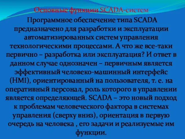 Основные функции SCADA-систем
 Ярмарка молодых специалистов МГГУ Математик-системный программист - 2012
 Распределенные системы. Лекция 1
 Виды информации и способы её представления
 Создание Web-сайта. Коммуникационные технологии
 3D принтеры
 Аналитические операции в ГИС (геоинформационные системы)
 Перевод чисел в системе счисления с основанием 2, 8, 16
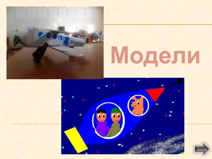 Урок информатики в 7 классе Модели и их назначение
 Введение в SMM. Урок №1
 Структура курсового проекта
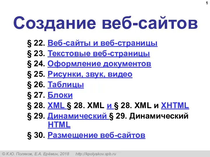 Создание веб-сайтов (§22-30). 11 класс
 Wetalk. Muammo
 Информационные ресурсы. (Лекция 4)
 Условный оператор в Паскале. 9 класс
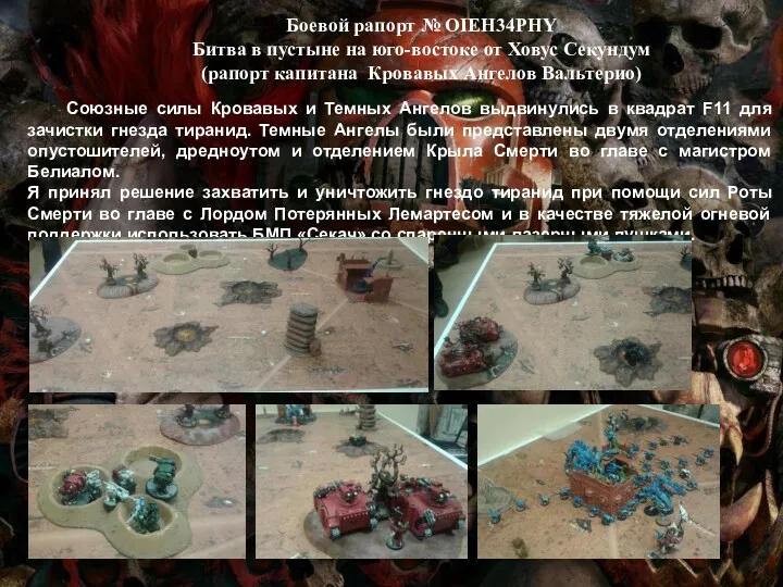 Битва в пустыне на юго-востоке от Ховус Секундум
 Социальные сети и их возможности
 Структура программы в Паскале. Ввод и вывод данных. (Тема 2)
 Базы данных и SQL. Семинар 4
 Презентация Microsoft PowerPoint (2)
 Моделирование, как метод познания. Формализация
 Забезпечення інформаційної безпеки інформаційно-телекомунікаційних систем на матеріалах в/ч А1815
 Базис языка визуального моделирования
 Europass. Login and two-factor authentication
 Основы языка HTML
 Текстовые редакторы. 8 класс
 Управление памятью. Функции ОC по управлению памятью