- Cmpe 466 computer graphics. 2D viewing. (Chapter 8)

Содержание
- 2. Window-to-viewport transformation Clipping window: section of 2D scene selected for display Viewport: window where the scene
- 3. Viewing pipeline Figure 8-2 Two-dimensional viewing-transformation pipeline. Normalization makes viewing device independent Clipping can be applied
- 4. Viewing coordinates Figure 8-3 A rotated clipping window defined in viewing coordinates.
- 5. Viewing coordinates Figure 8-4 A viewing-coordinate frame is moved into coincidence with the world frame by
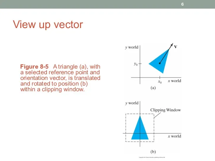
- 6. View up vector Figure 8-5 A triangle (a), with a selected reference point and orientation vector,
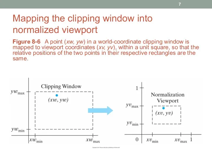
- 7. Mapping the clipping window into normalized viewport Figure 8-6 A point (xw, yw) in a world-coordinate
- 8. Window-to-viewport mapping
- 9. Window-to-viewport mapping
- 10. Alternative: mapping clipping window into a normalized square Advantage: clipping algorithms are standardized (see more later)
- 11. Mapping to a normalized square
- 12. Finally, mapping to viewport
- 13. Screen, display window, viewport Figure 8-8 A viewport at coordinate position (xs , ys ) within
- 14. OpenGL 2D viewing functions GLU clipping-window function OpenGL viewport function
- 15. Creating a GLUT display window
- 16. Example
- 17. Example
- 18. Example
- 19. 2D point clipping
- 20. 2D line clipping Figure 8-9 Clipping straight-line segments using a standard rectangular clipping window.
- 21. 2D line clipping: basic approach Test if line is completely inside or outside When both endpoints
- 22. Finding intersections and parametric equations
- 23. Parametric equations and clipping
- 24. Cohen-Sutherland line clipping Perform more tests before finding intersections Every line endpoint is assigned a 4-digit
- 25. Region codes Figure 8-10 A possible ordering for the clipping window boundaries corresponding to the bit
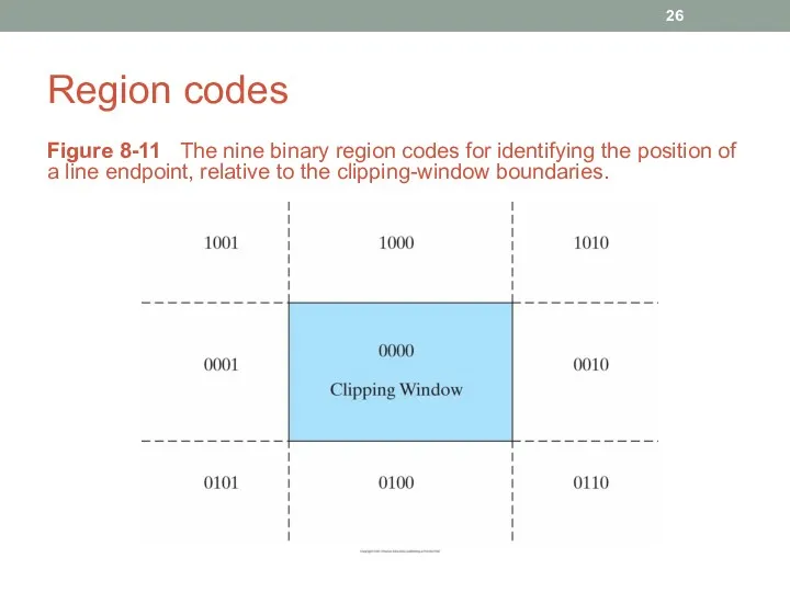
- 26. Region codes Figure 8-11 The nine binary region codes for identifying the position of a line
- 27. Cohen-Sutherland line clipping: steps Calculate differences between endpoint coordinates and clipping boundaries Use the resultant sign
- 28. Cohen-Sutherland line clipping: inside-outside tests For performance improvement, first do inside-outside tests When the OR operation
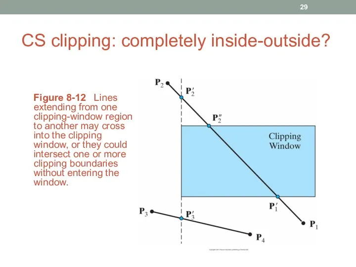
- 29. CS clipping: completely inside-outside? Figure 8-12 Lines extending from one clipping-window region to another may cross
- 30. CS clipping To determine whether the line crosses a selected clipping boundary, we check the corresponding
- 31. CS clipping where x value is set to either xwmin or xwmax, and the slope m=(yEnd-y0)/(xEnd-x0)
- 32. Liang-Barsky line clipping
- 33. Liang-Barsky line clipping (left) (right) (bottom) (top)
- 34. Liang-Barsky line clipping If pk=0 (line parallel to clipping window edge) If qk If qk≥0, the
- 35. LB algorithm If pk=0 and qk For all k such that pk For all k such
- 36. Notes LB is more efficient than CS Both CS and LB can be extended to 3D
- 37. Polygon Fill-Area Clipping Sutherland-Hodgman polygon clipping Figure 8-24 The four possible outputs generated by the left
- 38. Sutherland-Hodgman polygon clipping Figure 8-25 Processing a set of polygon vertices, {1, 2, 3}, through the
- 39. Sutherland-Hodgman polygon clipping Send pair of endpoints for each successive polygon line segment through the series
- 40. Sutherland-Hodgman polygon clipping The last clipper in this series generates a vertex list that describes the
- 42. Скачать презентацию
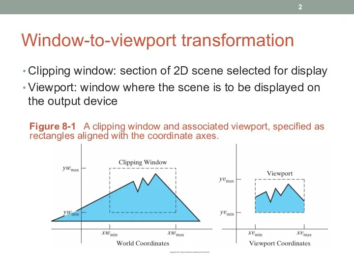
Window-to-viewport transformation
Clipping window: section of 2D scene selected for display
Viewport: window
Window-to-viewport transformation
Clipping window: section of 2D scene selected for display
Viewport: window
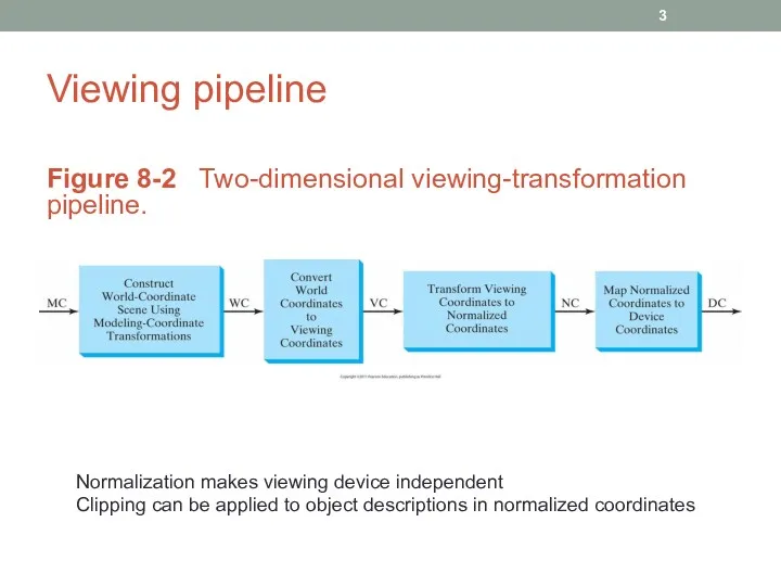
Viewing pipeline
Figure 8-2 Two-dimensional viewing-transformation pipeline.
Normalization makes viewing device independent
Clipping can
Viewing pipeline
Figure 8-2 Two-dimensional viewing-transformation pipeline.
Normalization makes viewing device independent
Clipping can
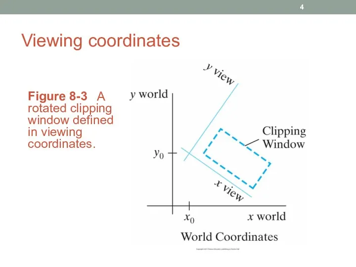
Viewing coordinates
Figure 8-3 A rotated clipping window defined in viewing coordinates.
Viewing coordinates
Figure 8-3 A rotated clipping window defined in viewing coordinates.
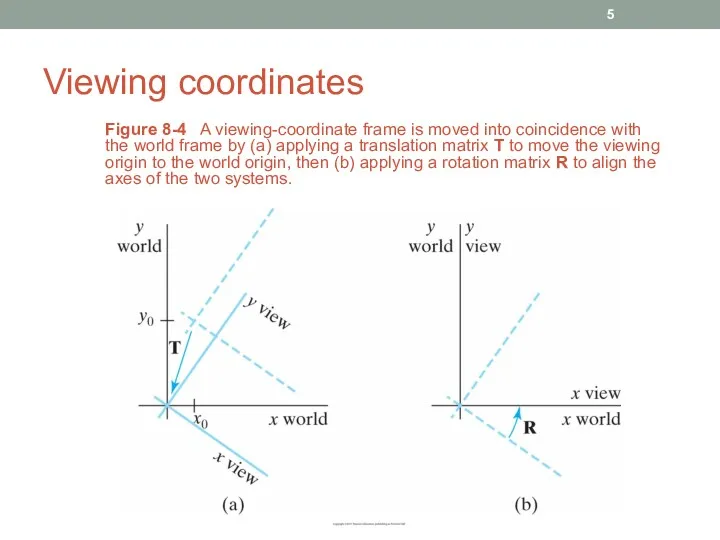
Viewing coordinates
Figure 8-4 A viewing-coordinate frame is moved into coincidence with
Viewing coordinates
Figure 8-4 A viewing-coordinate frame is moved into coincidence with
View up vector
Figure 8-5 A triangle (a), with a selected reference
View up vector
Figure 8-5 A triangle (a), with a selected reference
Mapping the clipping window into normalized viewport
Figure 8-6 A point (xw,
Mapping the clipping window into normalized viewport
Figure 8-6 A point (xw,
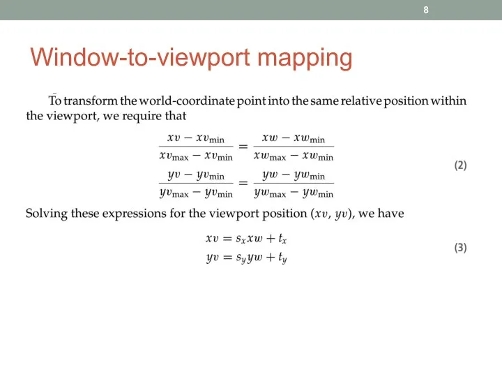
Window-to-viewport mapping
Window-to-viewport mapping
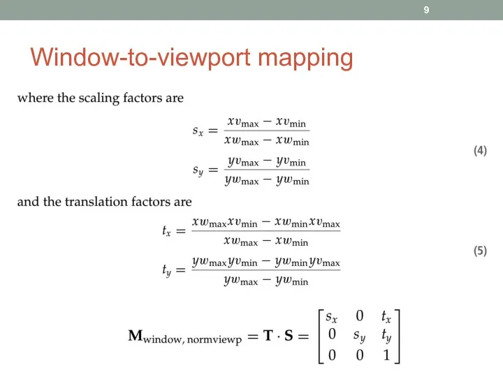
Window-to-viewport mapping
Window-to-viewport mapping
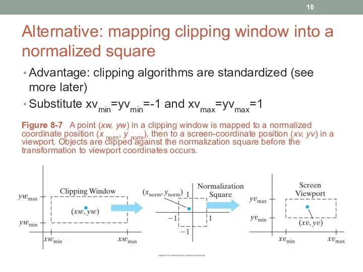
Alternative: mapping clipping window into a normalized square
Advantage: clipping algorithms are
Alternative: mapping clipping window into a normalized square
Advantage: clipping algorithms are
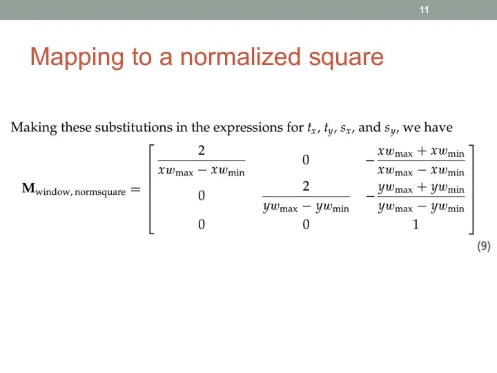
Mapping to a normalized square
Mapping to a normalized square
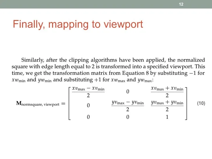
Finally, mapping to viewport
Finally, mapping to viewport
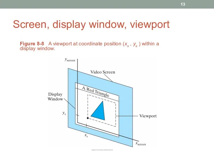
Screen, display window, viewport
Figure 8-8 A viewport at coordinate position (xs
Screen, display window, viewport
Figure 8-8 A viewport at coordinate position (xs
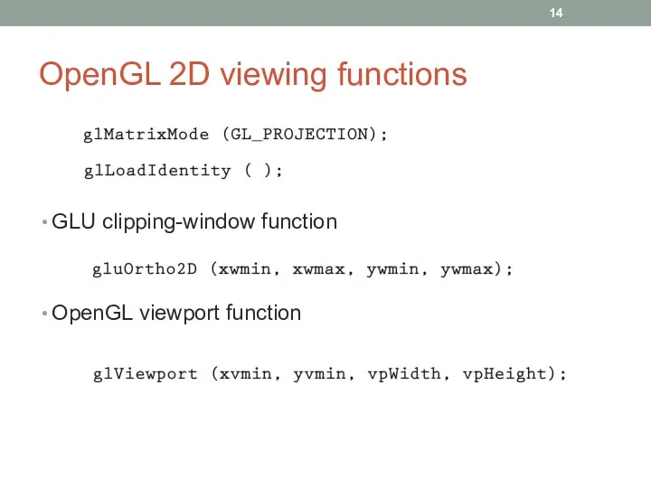
OpenGL 2D viewing functions
GLU clipping-window function
OpenGL viewport function
OpenGL 2D viewing functions
GLU clipping-window function
OpenGL viewport function
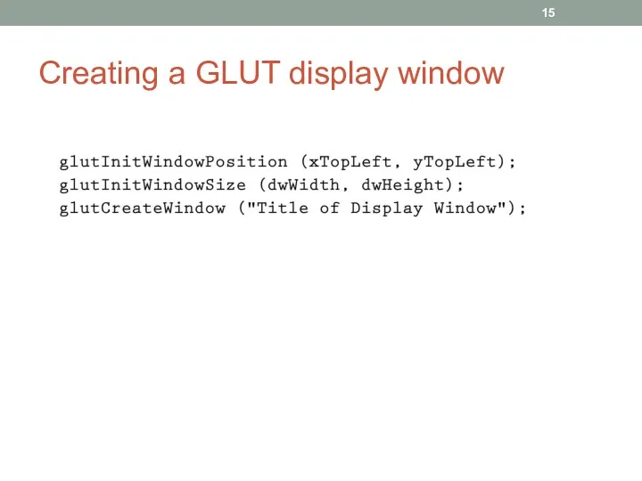
Creating a GLUT display window
Creating a GLUT display window
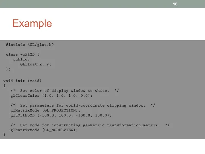
Example
Example
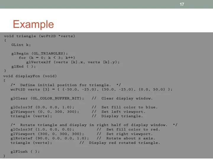
Example
Example
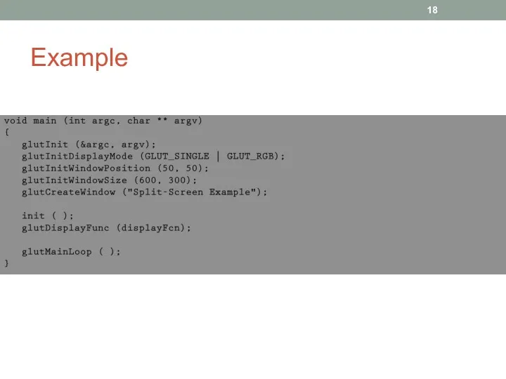
Example
Example
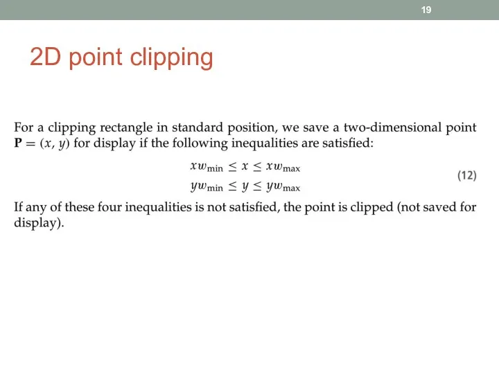
2D point clipping
2D point clipping
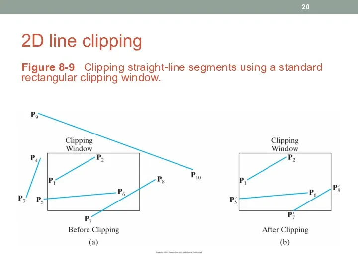
2D line clipping
Figure 8-9 Clipping straight-line segments using a standard rectangular
2D line clipping
Figure 8-9 Clipping straight-line segments using a standard rectangular
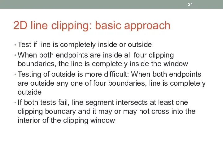
2D line clipping: basic approach
Test if line is completely inside or
2D line clipping: basic approach
Test if line is completely inside or
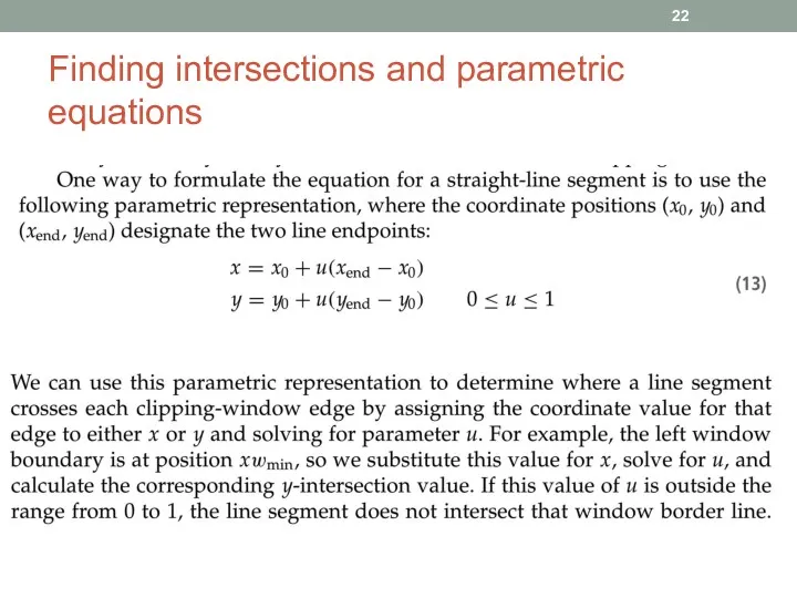
Finding intersections and parametric equations
Finding intersections and parametric equations
Parametric equations and clipping
Parametric equations and clipping
Cohen-Sutherland line clipping
Perform more tests before finding intersections
Every line endpoint is
Cohen-Sutherland line clipping
Perform more tests before finding intersections
Every line endpoint is
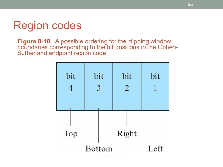
Region codes
Figure 8-10 A possible ordering for the clipping window boundaries
Region codes
Figure 8-10 A possible ordering for the clipping window boundaries
Region codes
Figure 8-11 The nine binary region codes for identifying the
Region codes
Figure 8-11 The nine binary region codes for identifying the
Cohen-Sutherland line clipping: steps
Calculate differences between endpoint coordinates and clipping boundaries
Use
Cohen-Sutherland line clipping: steps
Calculate differences between endpoint coordinates and clipping boundaries
Use
Cohen-Sutherland line clipping: inside-outside tests
For performance improvement, first do inside-outside tests
When
Cohen-Sutherland line clipping: inside-outside tests
For performance improvement, first do inside-outside tests
When
CS clipping: completely inside-outside?
Figure 8-12 Lines extending from one clipping-window region
CS clipping: completely inside-outside?
Figure 8-12 Lines extending from one clipping-window region
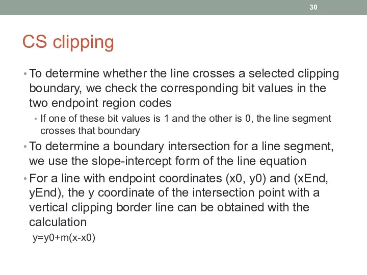
CS clipping
To determine whether the line crosses a selected clipping boundary,
CS clipping
To determine whether the line crosses a selected clipping boundary,
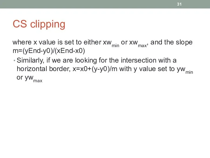
CS clipping
where x value is set to either xwmin or xwmax,
CS clipping
where x value is set to either xwmin or xwmax,
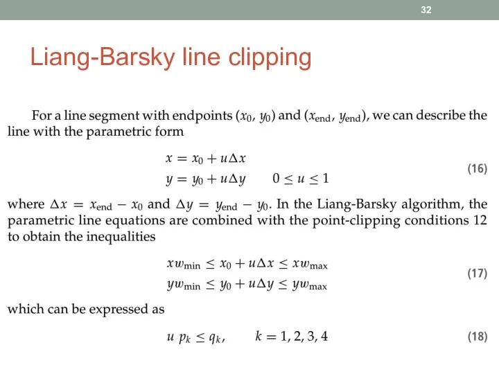
Liang-Barsky line clipping
Liang-Barsky line clipping
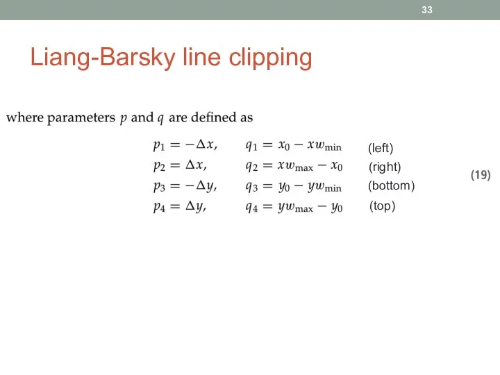
Liang-Barsky line clipping
(left)
(right)
(bottom)
(top)
Liang-Barsky line clipping
(left)
(right)
(bottom)
(top)
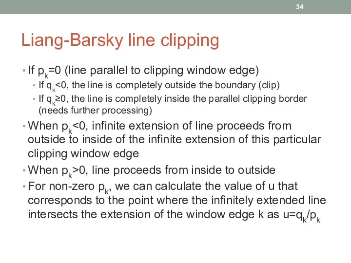
Liang-Barsky line clipping
If pk=0 (line parallel to clipping window edge)
If qk<0,
Liang-Barsky line clipping
If pk=0 (line parallel to clipping window edge)
If qk<0,
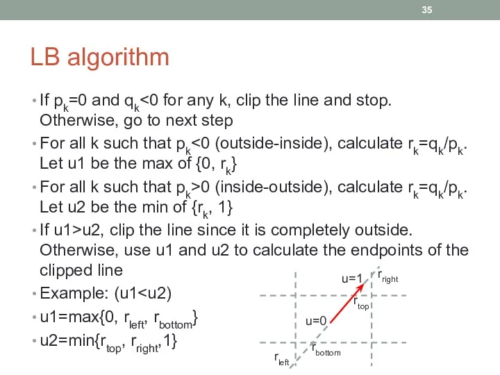
LB algorithm
If pk=0 and qk<0 for any k, clip the line
LB algorithm
If pk=0 and qk<0 for any k, clip the line
Notes
LB is more efficient than CS
Both CS and LB can be
Notes
LB is more efficient than CS
Both CS and LB can be
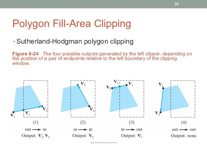
Polygon Fill-Area Clipping
Sutherland-Hodgman polygon clipping
Figure 8-24 The four possible outputs generated
Polygon Fill-Area Clipping
Sutherland-Hodgman polygon clipping
Figure 8-24 The four possible outputs generated
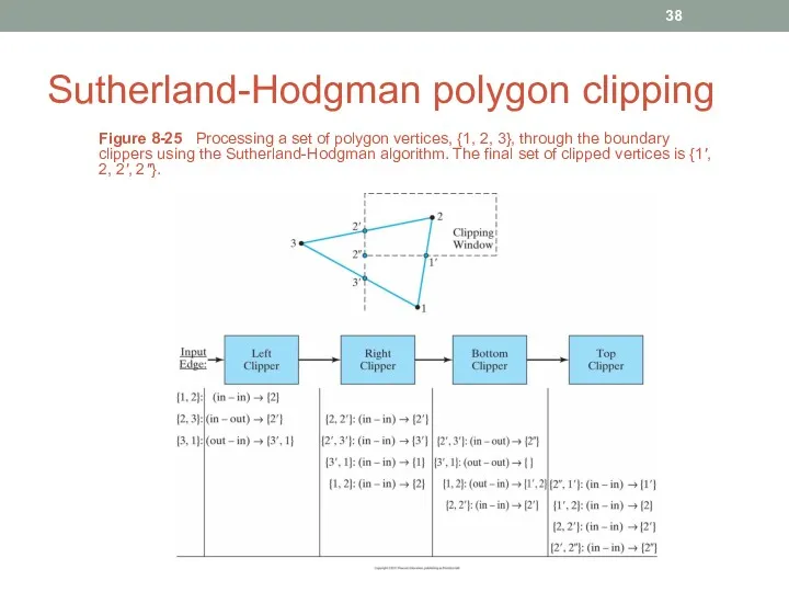
Sutherland-Hodgman polygon clipping
Figure 8-25 Processing a set of polygon vertices, {1,
Sutherland-Hodgman polygon clipping
Figure 8-25 Processing a set of polygon vertices, {1,
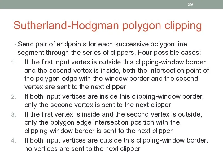
Sutherland-Hodgman polygon clipping
Send pair of endpoints for each successive polygon line
Sutherland-Hodgman polygon clipping
Send pair of endpoints for each successive polygon line
Sutherland-Hodgman polygon clipping
The last clipper in this series generates a vertex
Sutherland-Hodgman polygon clipping
The last clipper in this series generates a vertex
 Алгоритмы обработки информации. Алгоритмический этюд Перевозчик
 Инструкция по регистрации в Электронно-Библиотечной Системе ibooks.ru
 Социальная память. Функция социальной памяти
 Морская кибербезопасность в Российской Федерации
 Вредоносные и антивирусные программы
 Повторное использование кода. Наследование
 Дорожные знаки. Знаки сервиса
 Автоматизированные аналитико-статистические информационные системы, системы учета и управления
 Standard Controls Validation
 Разработка методов и алгоритмов для распознавания рукописных цифр с использованием нейронной сети
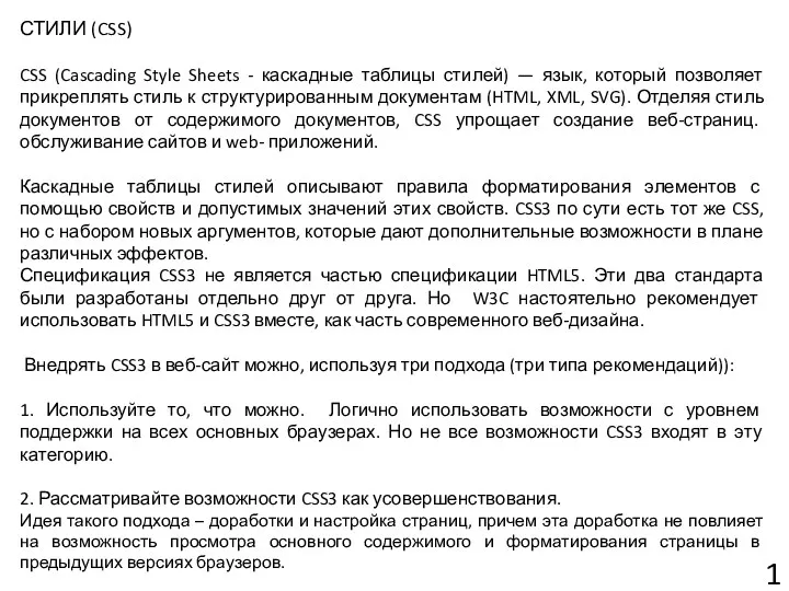 Стили (CSS)
 Техническое задание для создания сайта. Описание структуры
 Информационная безопасность несовершеннолетних
 Формы мышления. Алгебра высказываний
 Система станционной телемеханики
 MVC в Android. Создание простейшего приложения
 Геоинформатика. Оверлейные операции (операции пространственного наложения)
 Метод та програмна система моделювання користувацького плейлісту для персоналізації та рекомендацій
 Курсы по тестированию IT LABS. Тестовый случай. (Урок 4)
 Исполнитель робот. Задание по информатике
 Доступ к базам данных
 Сравнительная характеристика операционной системы Windows XP и Vista (11 класс)
 Жадные алгоритмы
 Как я вижу свою будущую профессию связиста
 Отчет по оценке сайта в сервисе Яндекс.Толока
 Программная платформа Node js
 Мобильное приложение: Мой Волжск
 Таблицы в Word