- CS 4700: Foundations of Artificial Intelligence

Содержание
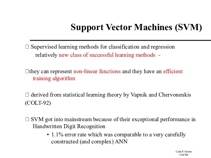
- 2. Support Vector Machines (SVM) ? Supervised learning methods for classification and regression relatively new class of
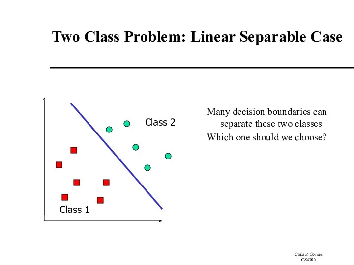
- 3. Two Class Problem: Linear Separable Case Class 1 Class 2 Many decision boundaries can separate these
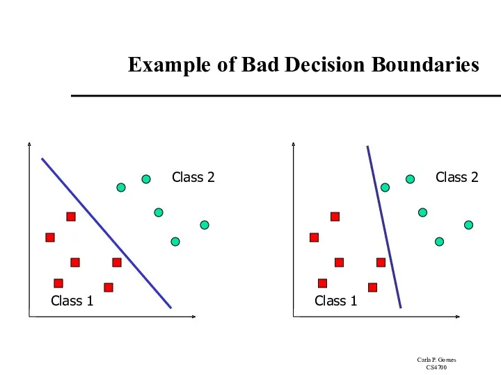
- 4. Example of Bad Decision Boundaries Class 1 Class 2 Class 1 Class 2
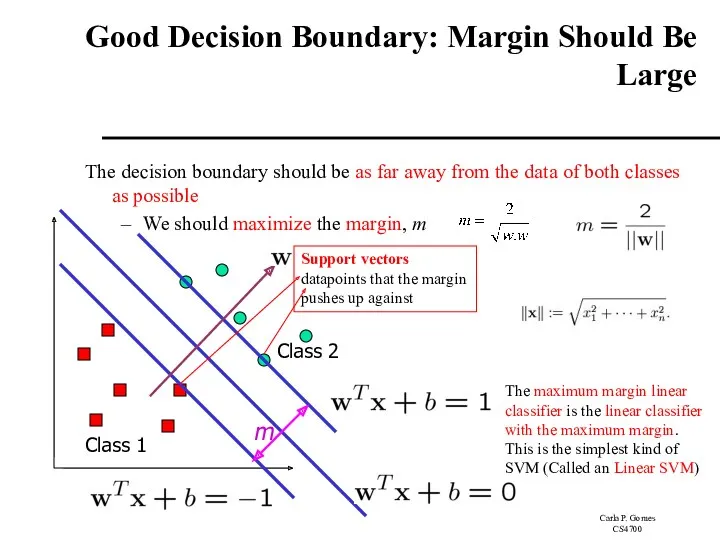
- 5. Good Decision Boundary: Margin Should Be Large The decision boundary should be as far away from
- 6. The Optimization Problem Let {x1, ..., xn} be our data set and let yi ∈ {1,-1}
- 7. Lagrangian of Original Problem The Lagrangian is Note that ||w||2 = wTw Setting the gradient of
- 8. The Dual Optimization Problem We can transform the problem to its dual This is a convex
- 9. α6=1.4 A Geometrical Interpretation Class 1 Class 2 α1=0.8 α2=0 α3=0 α4=0 α5=0 α7=0 α8=0.6 α9=0
- 10. Non-linearly Separable Problems We allow “error” ξi in classification; it is based on the output of
- 11. The Optimization Problem The dual of the problem is w is also recovered as The only
- 12. Extension to Non-linear SVMs (Kernel Machines)
- 13. Non-Linear SVM How could we generalize this procedure to non-linear data? Vapnik in 1992 showed that
- 14. Non-linear SVMs: Feature Space This slide is courtesy of www.iro.umontreal.ca/~pift6080/documents/papers/svm_tutorial.ppt If data are mapped into higher
- 15. Transformation to Feature Space Possible problem of the transformation High computation burden due to high-dimensionality and
- 16. Kernel Trick ☺ Recall: maximize subject to Since data is only represented as dot products, we
- 17. Example Transformation Consider the following transformation Define the kernel function K (x,y) as The inner product
- 18. Modification Due to Kernel Function Change all inner products to kernel functions For training, Original
- 19. Examples of Kernel Functions Polynomial kernel with degree d Radial basis function kernel with width σ
- 20. Example Suppose we have 5 1D data points x1=1, x2=2, x3=4, x4=5, x5=6, with 1, 2,
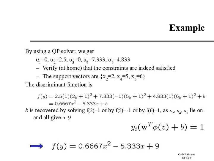
- 21. Example By using a QP solver, we get α1=0, α2=2.5, α3=0, α4=7.333, α5=4.833 Verify (at home)
- 22. Example Value of discriminant function 1 2 4 5 6 class 2 class 1 class 1
- 23. Choosing the Kernel Function Probably the most tricky part of using SVM. The kernel function is
- 24. Software A list of SVM implementation can be found at http://www.kernel-machines.org/software.html Some implementation (such as LIBSVM)
- 25. Recap of Steps in SVM Prepare data matrix {(xi,yi)} Select a Kernel function Select the error
- 26. Summary Weaknesses Training (and Testing) is quite slow compared to ANN Because of Constrained Quadratic Programming
- 27. Summary Strengths Training is relatively easy We don’t have to deal with local minimum like in
- 28. Applications of SVMs Bioinformatics Machine Vision Text Categorization Ranking (e.g., Google searches) Handwritten Character Recognition Time
- 29. Handwritten digit recognition
- 30. References Burges, C. “A Tutorial on Support Vector Machines for Pattern Recognition.” Bell Labs. 1998 Law,
- 32. Скачать презентацию
Support Vector Machines (SVM)
? Supervised learning methods for classification and
Support Vector Machines (SVM)
? Supervised learning methods for classification and
Two Class Problem: Linear Separable Case
Class 1
Class 2
Many decision boundaries can
Two Class Problem: Linear Separable Case
Class 1
Class 2
Many decision boundaries can
Example of Bad Decision Boundaries
Class 1
Class 2
Class 1
Class 2
Example of Bad Decision Boundaries
Class 1
Class 2
Class 1
Class 2
Good Decision Boundary: Margin Should Be Large
The decision boundary should be
Good Decision Boundary: Margin Should Be Large
The decision boundary should be
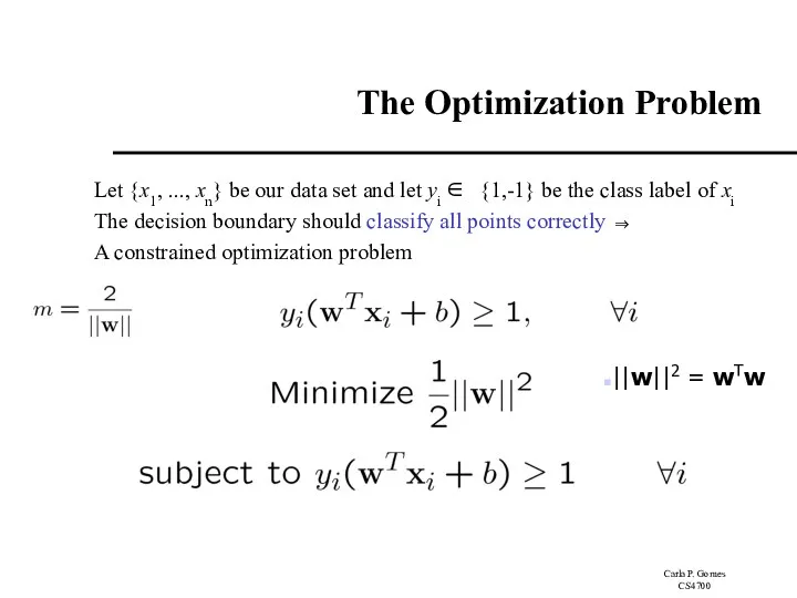
The Optimization Problem
Let {x1, ..., xn} be our data set and
The Optimization Problem
Let {x1, ..., xn} be our data set and
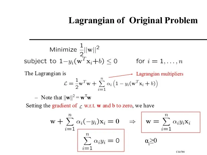
Lagrangian of Original Problem
The Lagrangian is
Note that ||w||2 = wTw
Setting
Lagrangian of Original Problem
The Lagrangian is
Note that ||w||2 = wTw
Setting
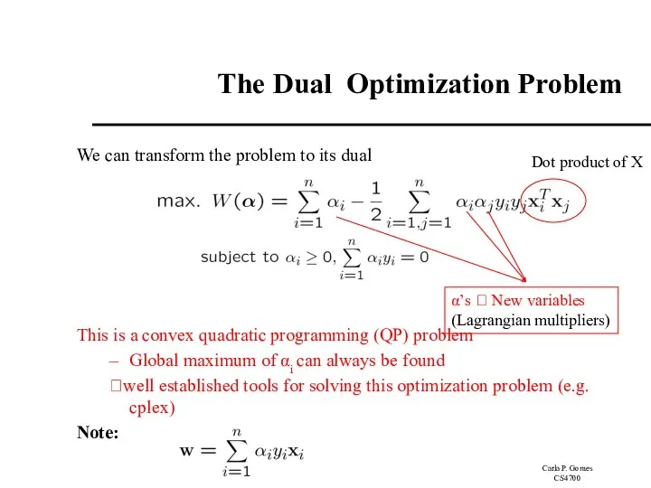
The Dual Optimization Problem
We can transform the problem to its dual
This
The Dual Optimization Problem
We can transform the problem to its dual
This
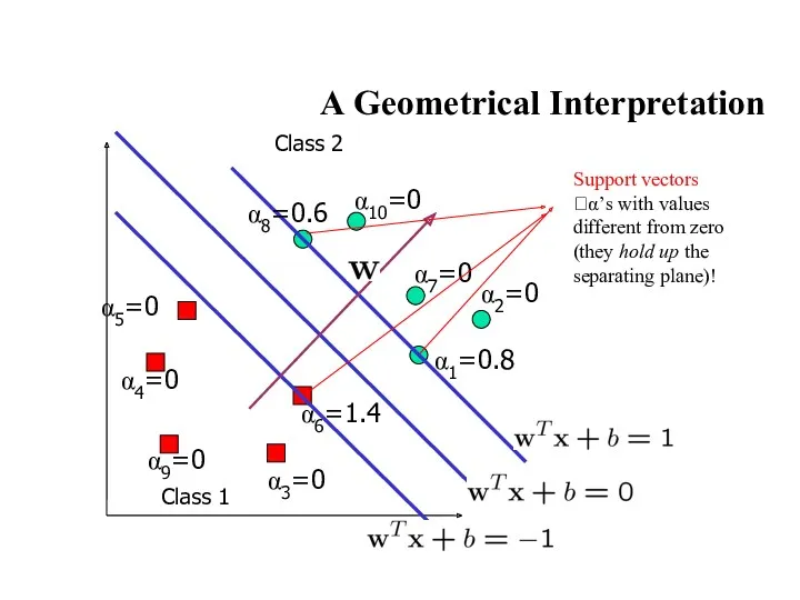
α6=1.4
A Geometrical Interpretation
Class 1
Class 2
α1=0.8
α2=0
α3=0
α4=0
α5=0
α7=0
α8=0.6
α9=0
α10=0
α6=1.4
A Geometrical Interpretation
Class 1
Class 2
α1=0.8
α2=0
α3=0
α4=0
α5=0
α7=0
α8=0.6
α9=0
α10=0
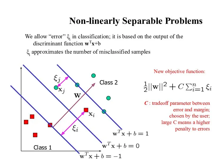
Non-linearly Separable Problems
We allow “error” ξi in classification; it is based
Non-linearly Separable Problems
We allow “error” ξi in classification; it is based
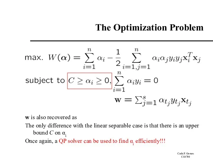
The Optimization Problem
The dual of the problem is
w is also recovered
The Optimization Problem
The dual of the problem is
w is also recovered
Extension to Non-linear SVMs
(Kernel Machines)
Extension to Non-linear SVMs
(Kernel Machines)
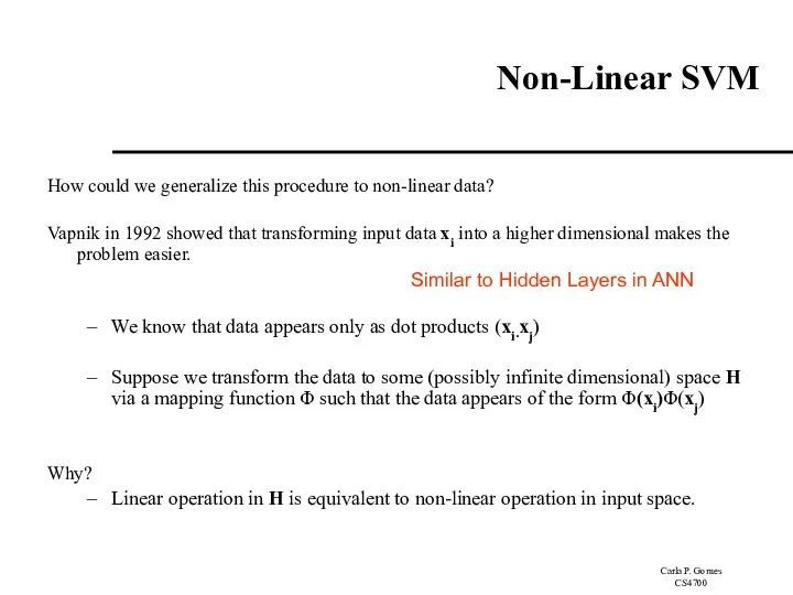
Non-Linear SVM
How could we generalize this procedure to non-linear data?
Vapnik in
Non-Linear SVM
How could we generalize this procedure to non-linear data?
Vapnik in
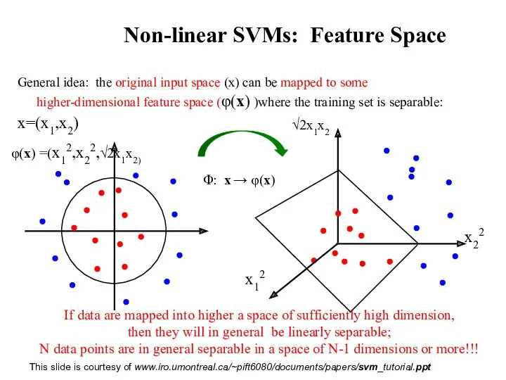
Non-linear SVMs: Feature Space
This slide is courtesy of www.iro.umontreal.ca/~pift6080/documents/papers/svm_tutorial.ppt
If data
Non-linear SVMs: Feature Space
This slide is courtesy of www.iro.umontreal.ca/~pift6080/documents/papers/svm_tutorial.ppt
If data
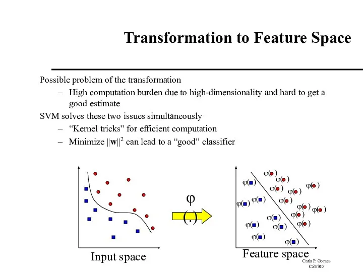
Transformation to Feature Space
Possible problem of the transformation
High computation burden due
Transformation to Feature Space
Possible problem of the transformation
High computation burden due
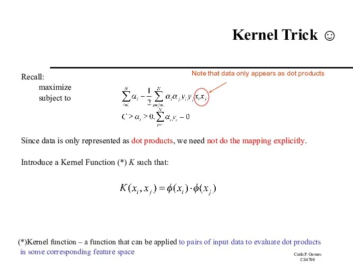
Kernel Trick ☺
Recall:
maximize
subject to
Since data is only represented as dot products,
Kernel Trick ☺
Recall:
maximize
subject to
Since data is only represented as dot products,
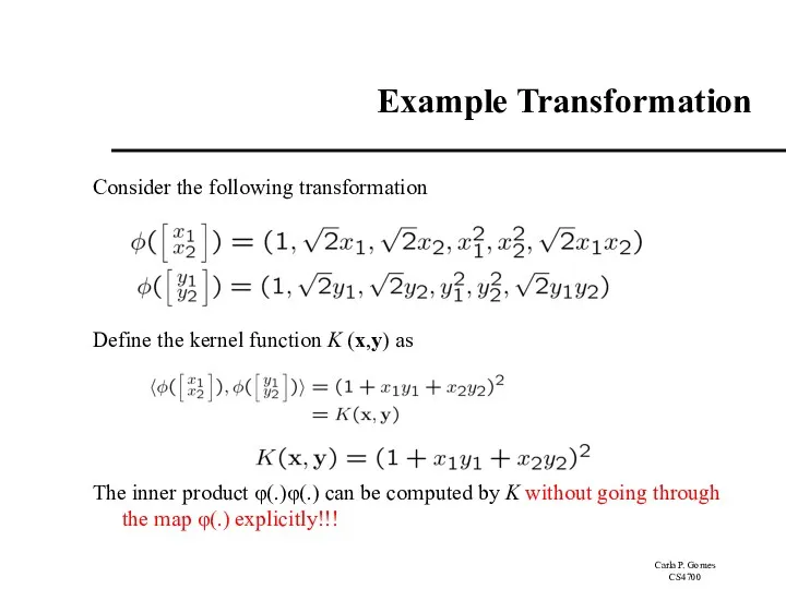
Example Transformation
Consider the following transformation
Define the kernel function K (x,y) as
Example Transformation
Consider the following transformation
Define the kernel function K (x,y) as
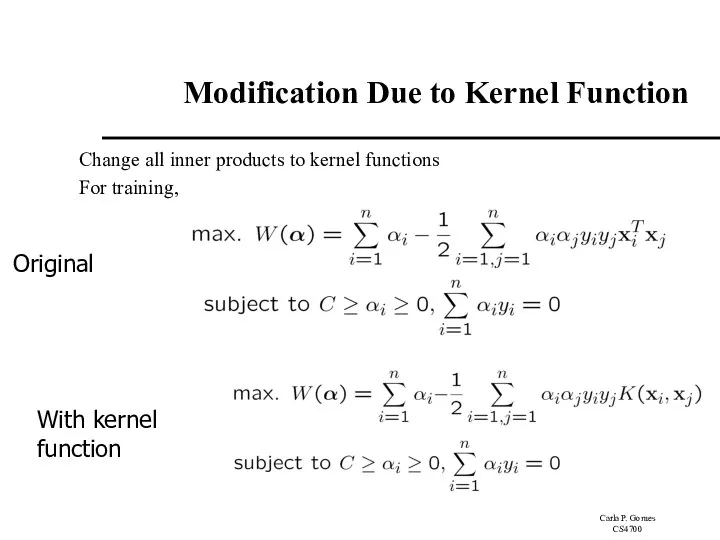
Modification Due to Kernel Function
Change all inner products to kernel functions
For
Modification Due to Kernel Function
Change all inner products to kernel functions
For
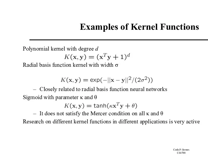
Examples of Kernel Functions
Polynomial kernel with degree d
Radial basis function kernel
Examples of Kernel Functions
Polynomial kernel with degree d
Radial basis function kernel
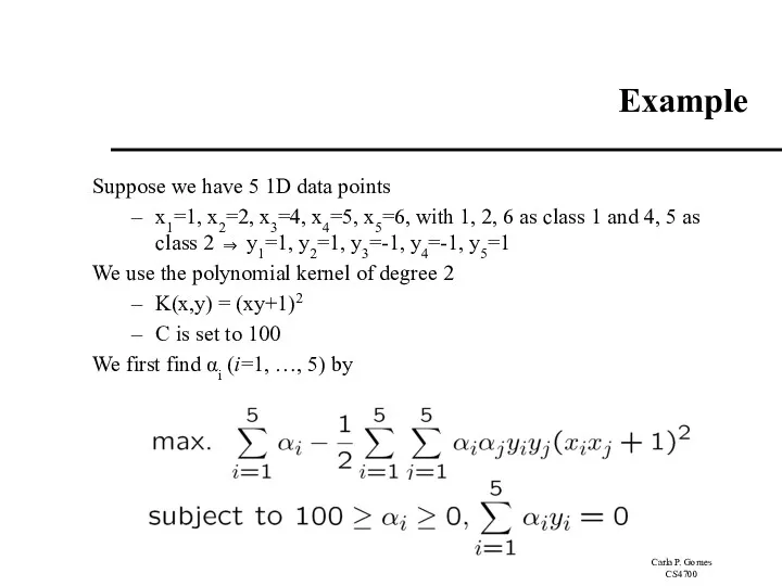
Example
Suppose we have 5 1D data points
x1=1, x2=2, x3=4, x4=5, x5=6,
Example
Suppose we have 5 1D data points
x1=1, x2=2, x3=4, x4=5, x5=6,
Example
By using a QP solver, we get
α1=0, α2=2.5, α3=0, α4=7.333, α5=4.833
Verify
Example
By using a QP solver, we get
α1=0, α2=2.5, α3=0, α4=7.333, α5=4.833
Verify
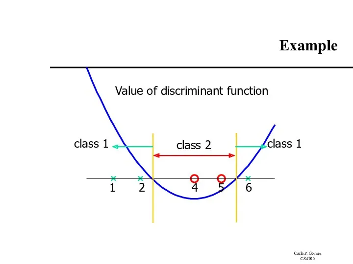
Example
Value of discriminant function
1
2
4
5
6
class 2
class 1
class 1
Example
Value of discriminant function
1
2
4
5
6
class 2
class 1
class 1
Choosing the Kernel Function
Probably the most tricky part of using SVM.
The
Choosing the Kernel Function
Probably the most tricky part of using SVM.
The
Software
A list of SVM implementation can be found at http://www.kernel-machines.org/software.html
Some implementation
Software
A list of SVM implementation can be found at http://www.kernel-machines.org/software.html
Some implementation
Recap of Steps in SVM
Prepare data matrix {(xi,yi)}
Select a Kernel function
Select
Recap of Steps in SVM
Prepare data matrix {(xi,yi)}
Select a Kernel function
Select
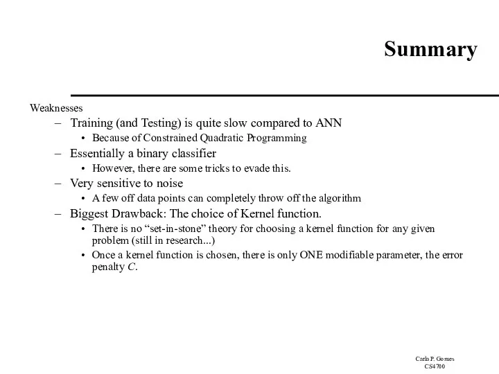
Summary
Weaknesses
Training (and Testing) is quite slow compared to ANN
Because of
Summary
Weaknesses
Training (and Testing) is quite slow compared to ANN
Because of
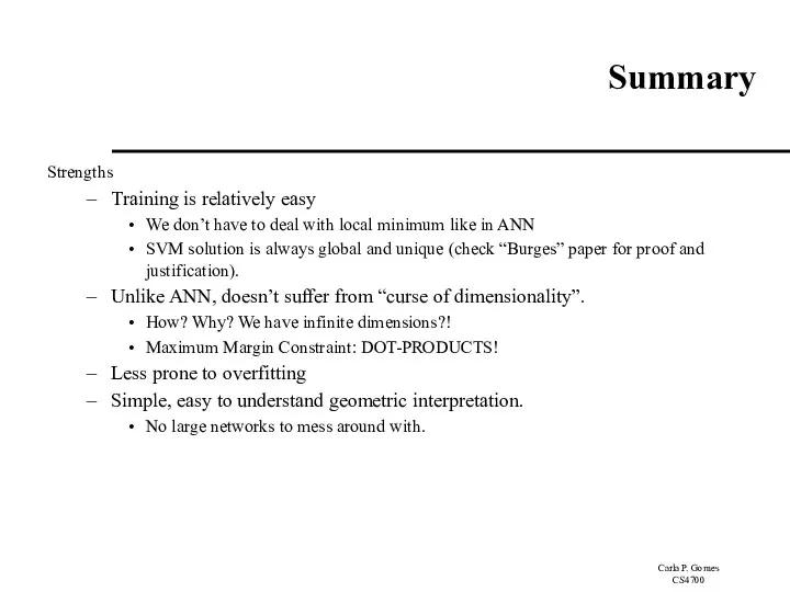
Summary
Strengths
Training is relatively easy
We don’t have to deal with local minimum
Summary
Strengths
Training is relatively easy
We don’t have to deal with local minimum
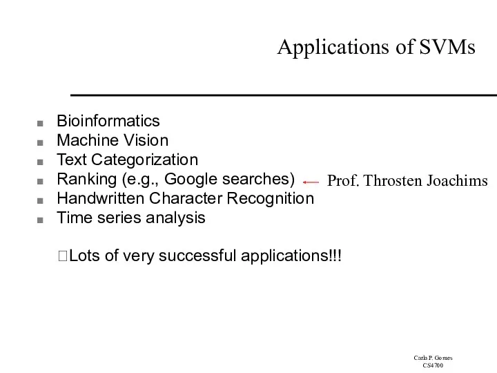
Applications of SVMs
Bioinformatics
Machine Vision
Text Categorization
Ranking (e.g., Google searches)
Handwritten Character Recognition
Time series
Applications of SVMs
Bioinformatics
Machine Vision
Text Categorization
Ranking (e.g., Google searches)
Handwritten Character Recognition
Time series
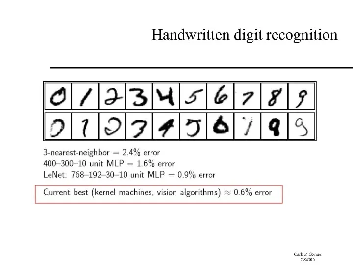
Handwritten digit recognition
Handwritten digit recognition
References
Burges, C. “A Tutorial on Support Vector Machines for Pattern Recognition.”
References
Burges, C. “A Tutorial on Support Vector Machines for Pattern Recognition.”
 Өз ойыным. 4 класс
 Использование графических браузеров
 Тернарный оператор: правила использования
 Процессор. Устройство управления
 Классы памяти и область действия объектов
 Инструкция пользования роботом
 Конспект урока с презентацией для 3 класса по теме Представление информации
 Язык гипертекстовой разметки HTML
 Компьютерная графика. Векторная графика. Фрактальная графика
 Java Script. Первое знакомство
 Виртуальная АТС. Экономичное и эффективное решение для организации офисной связи
 Создание сложной игры для двух игроков Мортал Комбат или Пираты Карибского моря
 Машина Тьюринга
 Структуры и объединения. Лекция 7
 Статистические методы обработки информации
 Представление информации в форме таблиц. Структура таблицы. Информатика. 5 класс
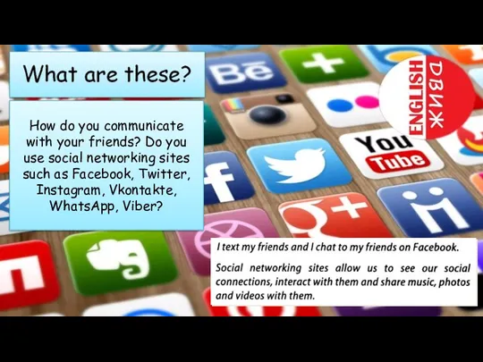 How do you communicate with your friends?
 Некоторые системотехнические аспекты оценки эффективности функционирования ситуационных центров
 Алгоритми. Складність алгоритмів. Алгоритм бінарного пошуку
 Организация работы психолога в удаленном режиме
 Газета Ровесник. Март 2016
 Karmarkar Algorithm
 Совершенствование управления деятельностью кредитной организации на основе применения технологии искусственного интеллекта
 Сортировка массивов. Основы программирования
 Manual QA course. Базы данных ( Lecture 16.1)
 Кодирование. Оптимальный код Хаффмана. Лекция 14
 ava Lecture DB. JDBC
 Предметная область базы данных