- Dynamic Programming

Содержание
- 4. Dynamic Programming Dynamic programming is a very powerful, general tool for solving optimization problems. Once understood
- 5. Greedy Algorithms Greedy algorithms focus on making the best local choice at each decision point. For
- 6. Problem: Let’s consider the calculation of Fibonacci numbers: F(n) = F(n-2) + F(n-1) with seed values
- 7. Recursive Algorithm: Fib(n) { if (n == 0) return 0; if (n == 1) return 1;
- 8. Recursive Algorithm: Fib(n) { if (n == 0) return 0; if (n == 1) return 1;
- 9. Recursion tree What’s the problem?
- 10. Memoization: Fib(n) { if (n == 0) return M[0]; if (n == 1) return M[1]; if
- 11. already calculated …
- 12. Dynamic programming - Main approach: recursive, holds answers to a sub problem in a table, can
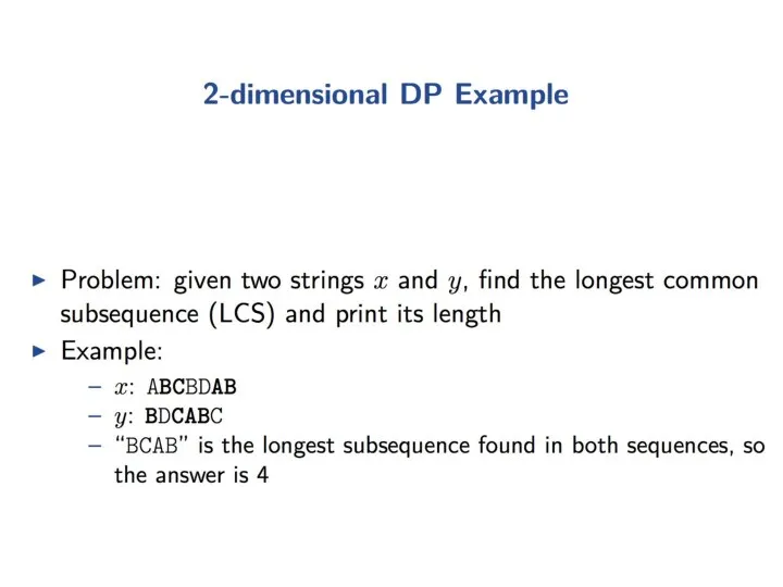
- 13. 1-dimensional DP Problem
- 14. 1-dimensional DP Problem
- 15. 1-dimensional DP Problem
- 16. 1-dimensional DP Problem
- 17. What happens when n is extremely large?
- 21. Tri Tiling
- 22. Tri Tiling
- 23. Tri Tiling
- 25. Finding Recurrences
- 26. Finding Recurrences
- 27. Extension Solving the problem for n x m grids, where n is small, say n ≤
- 29. Egg dropping problem
- 30. Egg dropping problem
- 31. Egg dropping problem
- 32. Egg dropping problem
- 33. Egg dropping problem
- 34. Egg dropping problem
- 35. Egg dropping problem
- 36. Egg dropping problem(n eggs) Dynamic Programming Approach D[j,m] : There are j floors and m eggs.
- 37. Egg dropping problem(n eggs) Dynamic Programming Approach DP[j,m] : There are j floors and m eggs.
- 38. Egg dropping problem(n eggs) Dynamic Programming Approach DP[j,m] : There are j floors and m eggs.
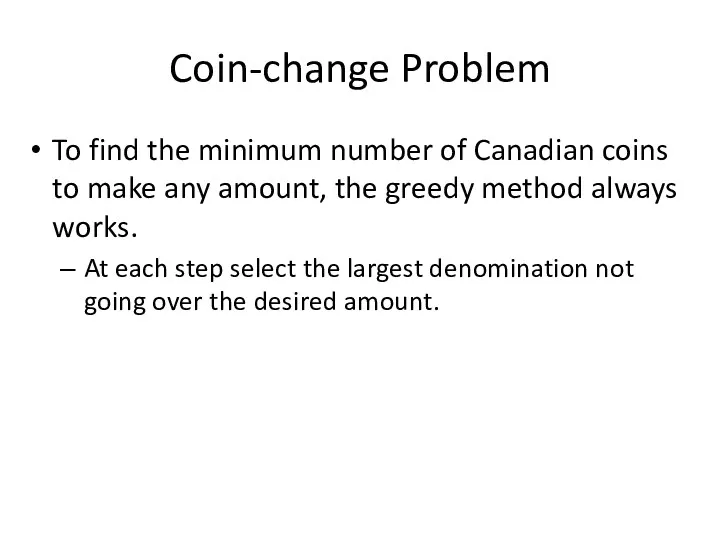
- 48. Coin-change Problem To find the minimum number of Canadian coins to make any amount, the greedy
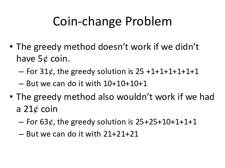
- 49. Coin-change Problem The greedy method doesn’t work if we didn’t have 5¢ coin. For 31¢, the
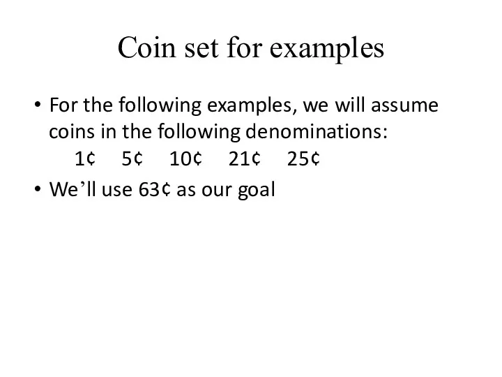
- 50. Coin set for examples For the following examples, we will assume coins in the following denominations:
- 51. A solution We can reduce the problem recursively by choosing the first coin, and solving for
- 52. A dynamic programming solution Idea: Solve first for one cent, then two cents, then three cents,
- 53. A dynamic programming solution Let T(n) be the number of coins taken to dispense n¢. The
- 54. A dynamic programming solution The dynamic programming algorithm is O(N*K) where N is the desired amount
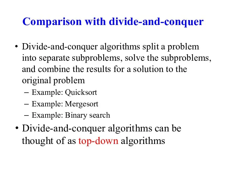
- 55. Comparison with divide-and-conquer Divide-and-conquer algorithms split a problem into separate subproblems, solve the subproblems, and combine
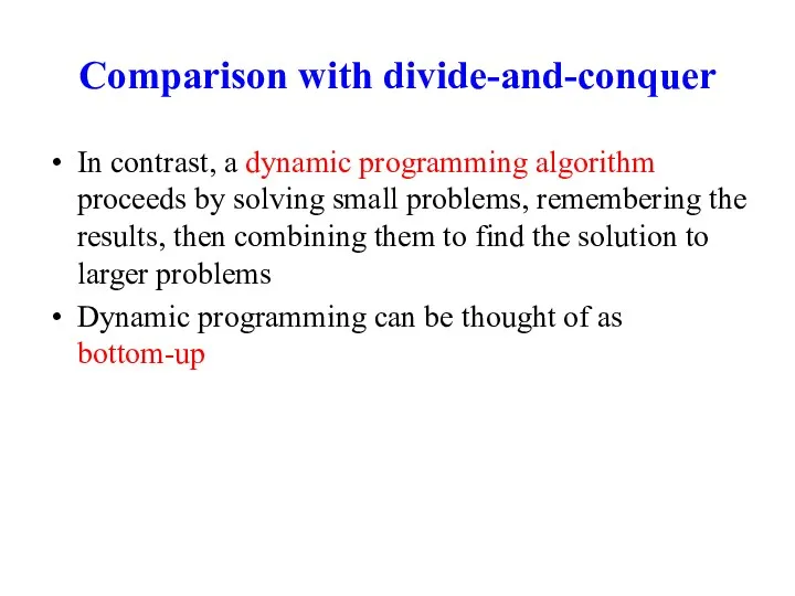
- 56. Comparison with divide-and-conquer In contrast, a dynamic programming algorithm proceeds by solving small problems, remembering the
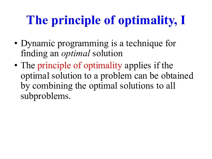
- 57. The principle of optimality, I Dynamic programming is a technique for finding an optimal solution The
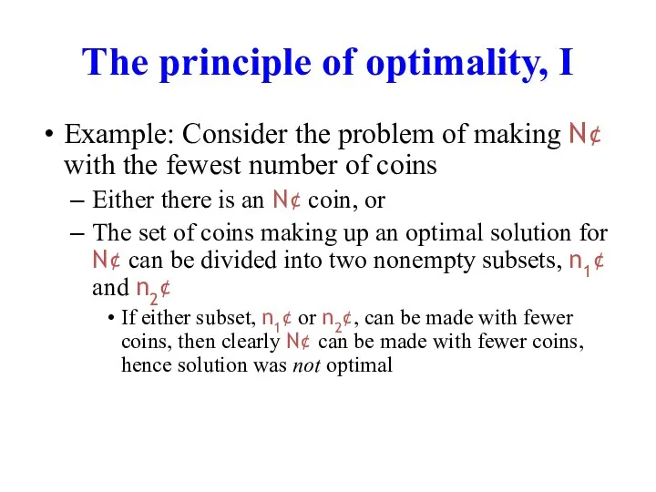
- 58. The principle of optimality, I Example: Consider the problem of making N¢ with the fewest number
- 59. The principle of optimality, II The principle of optimality holds if Every optimal solution to a
- 60. The principle of optimality, II Example: In coin problem, The optimal solution to 7¢ is 5¢
- 61. Longest simple path Consider the following graph: The longest simple path (path not containing a cycle)
- 62. Example: In coin problem, The optimal solution to 7¢ is 5¢ + 1¢ + 1¢, and
- 63. The 0-1 knapsack problem A thief breaks into a house, carrying a knapsack... He can carry
- 64. The 0-1 knapsack problem A greedy algorithm does not find an optimal solution A dynamic programming
- 65. The 0-1 knapsack problem This is similar to, but not identical to, the coins problem In
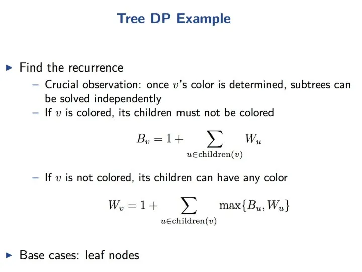
- 66. Steps for Solving DP Problems Define subproblems Write down the recurrence that relates subproblems Recognize and
- 67. Comments Dynamic programming relies on working “from the bottom up” and saving the results of solving
- 69. Скачать презентацию
Dynamic Programming
Dynamic programming is a very powerful, general tool for solving
Dynamic Programming
Dynamic programming is a very powerful, general tool for solving
Greedy Algorithms
Greedy algorithms focus on making the best local choice at
Greedy Algorithms
Greedy algorithms focus on making the best local choice at
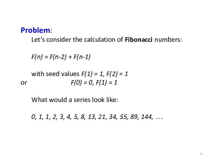
Problem:
Let’s consider the calculation of Fibonacci numbers:
F(n) = F(n-2) +
Problem:
Let’s consider the calculation of Fibonacci numbers:
F(n) = F(n-2) +
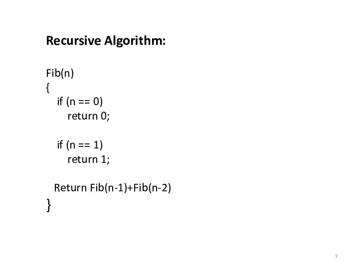
Recursive Algorithm:
Fib(n)
{
if (n == 0)
return 0;
if (n ==
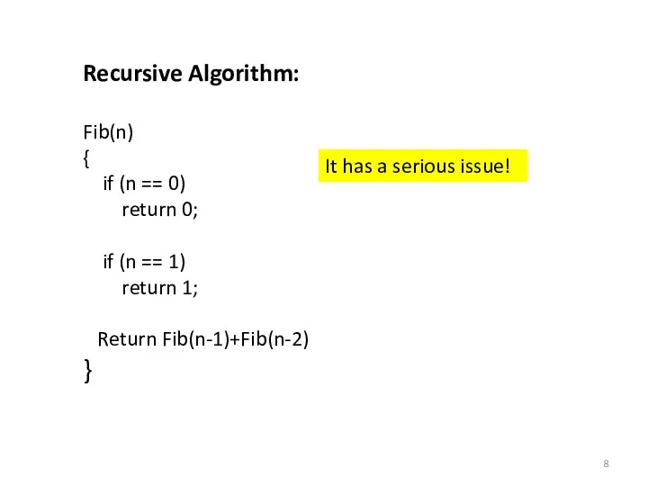
Recursive Algorithm:
Fib(n)
{
if (n == 0)
return 0;
if (n ==
Recursive Algorithm:
Fib(n)
{
if (n == 0)
return 0;
if (n ==
Recursive Algorithm:
Fib(n)
{
if (n == 0)
return 0;
if (n ==
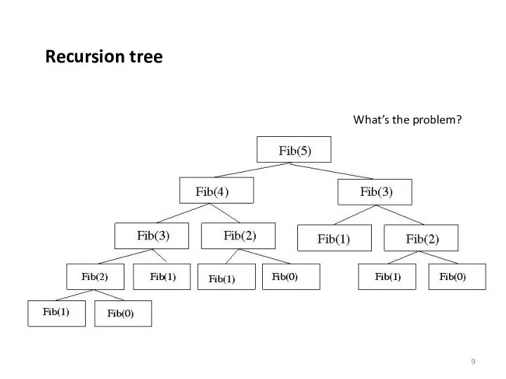
Recursion tree
What’s the problem?
Recursion tree
What’s the problem?
![Memoization: Fib(n) { if (n == 0) return M[0]; if](/_ipx/f_webp&q_80&fit_contain&s_1440x1080/imagesDir/jpg/598664/slide-9.jpg)
Memoization:
Fib(n)
{
if (n == 0)
return M[0];
if (n == 1)
Memoization:
Fib(n)
{
if (n == 0)
return M[0];
if (n == 1)
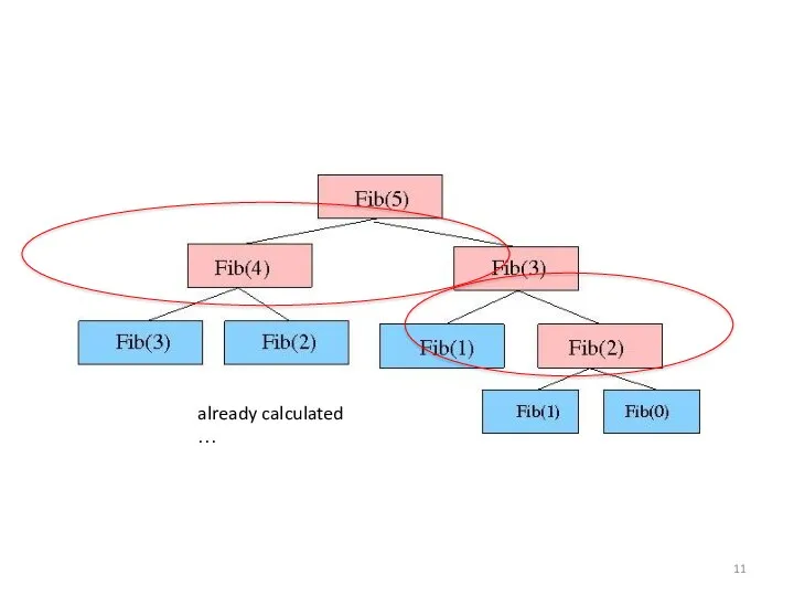
already calculated …
already calculated …
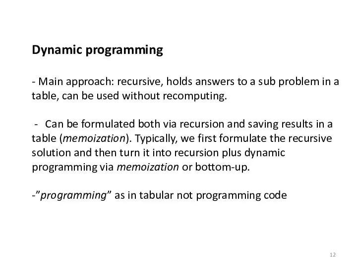
Dynamic programming
- Main approach: recursive, holds answers to a sub problem
Dynamic programming
- Main approach: recursive, holds answers to a sub problem
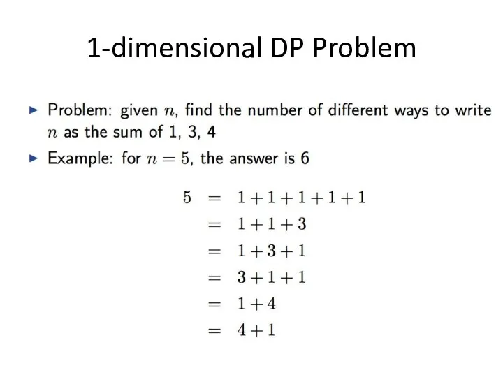
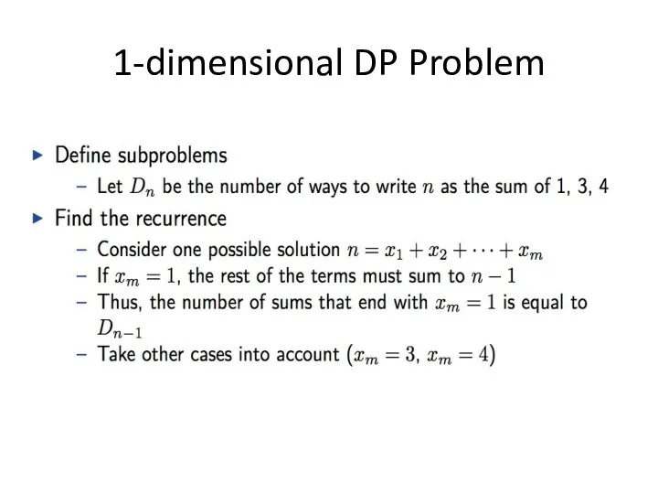
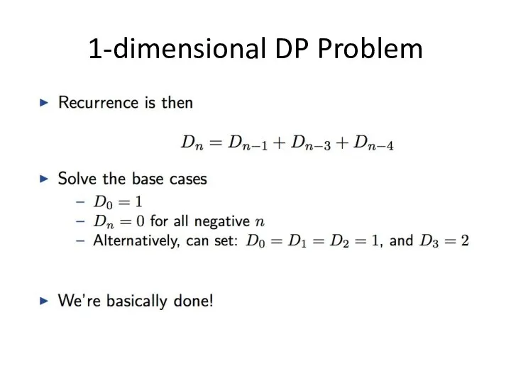
1-dimensional DP Problem
1-dimensional DP Problem
1-dimensional DP Problem
1-dimensional DP Problem
1-dimensional DP Problem
1-dimensional DP Problem
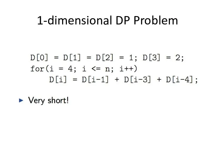
1-dimensional DP Problem
1-dimensional DP Problem
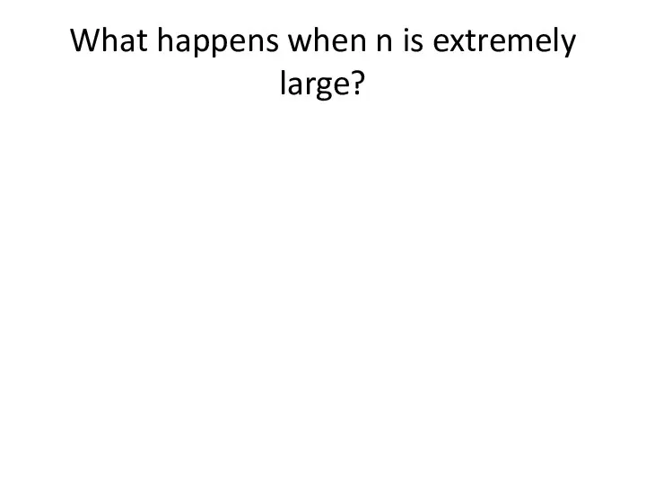
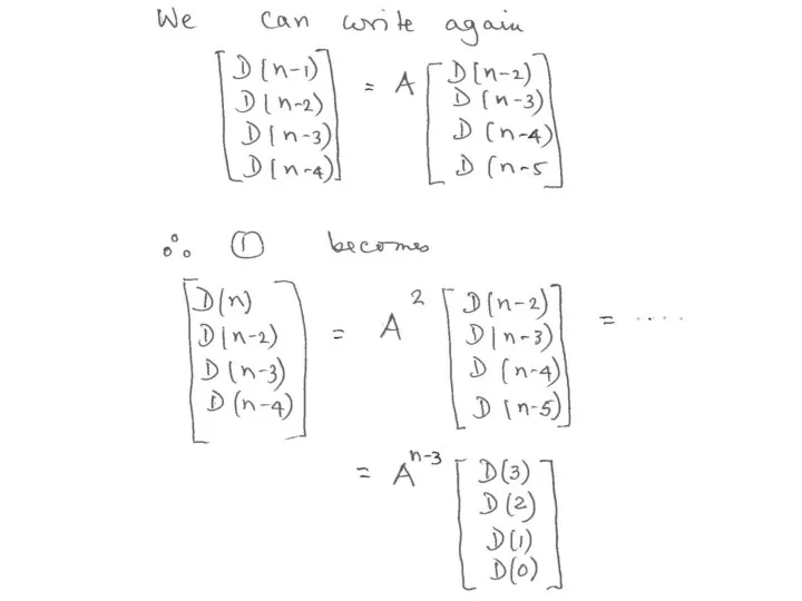
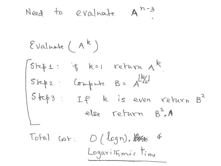
What happens when n is extremely large?
What happens when n is extremely large?
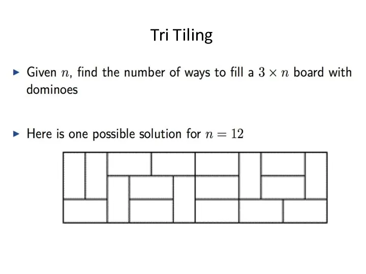
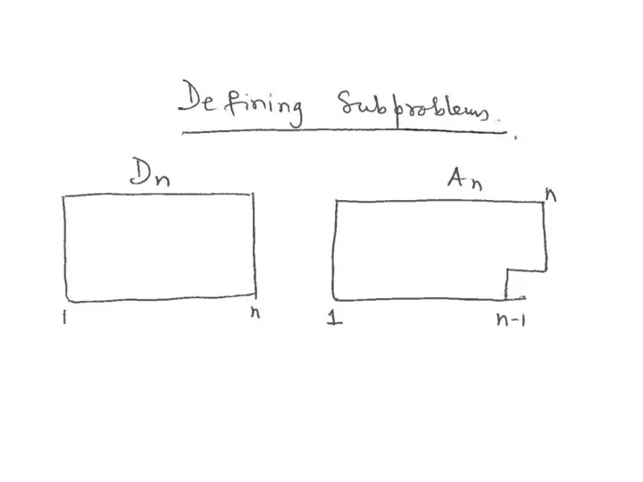
Tri Tiling
Tri Tiling
Tri Tiling
Tri Tiling
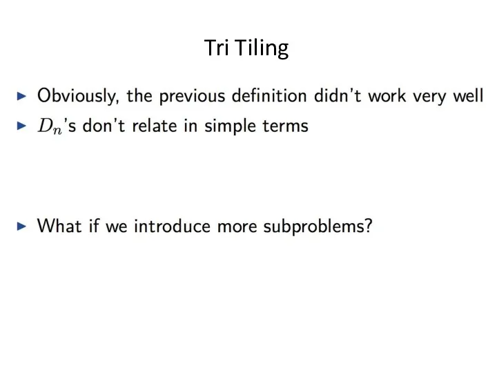
Tri Tiling
Tri Tiling
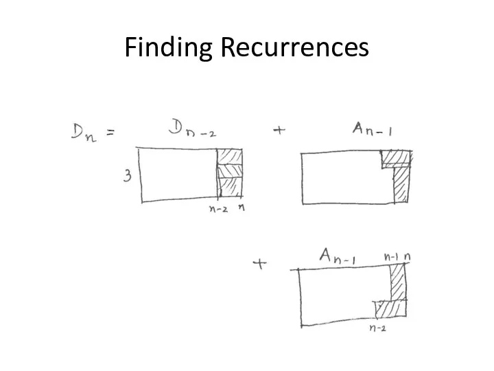
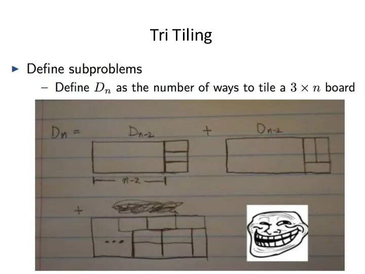
Finding Recurrences
Finding Recurrences
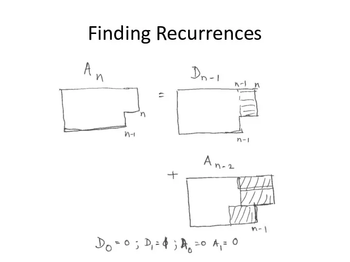
Finding Recurrences
Finding Recurrences
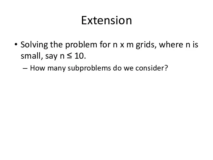
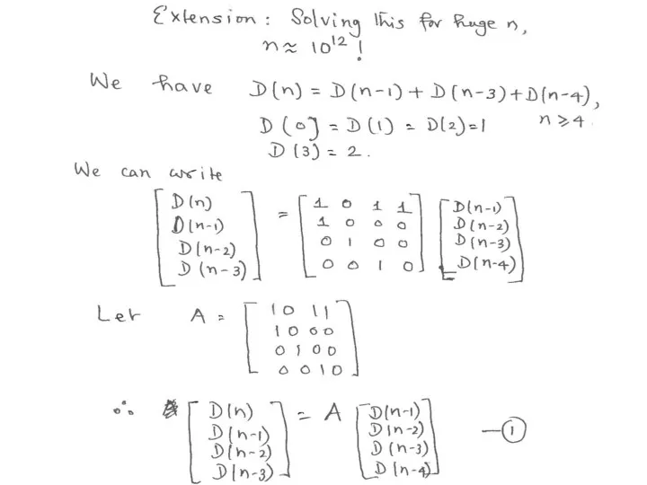
Extension
Solving the problem for n x m grids, where n is
Extension
Solving the problem for n x m grids, where n is

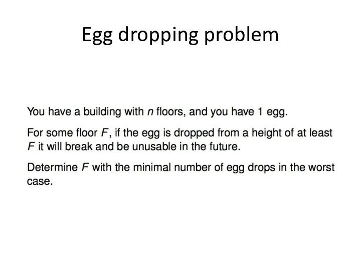
Egg dropping problem
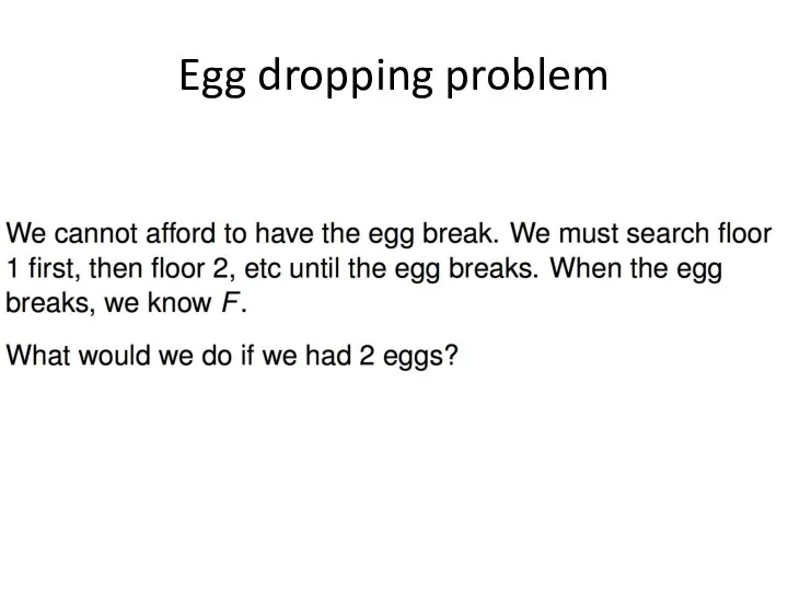
Egg dropping problem
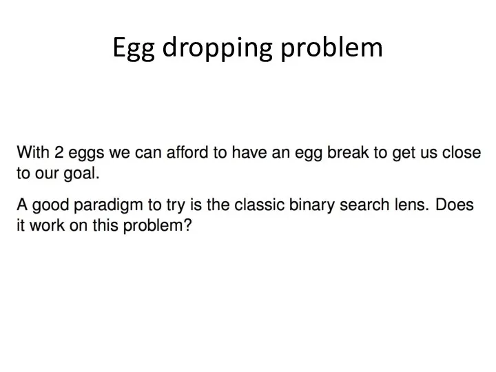
Egg dropping problem
Egg dropping problem
Egg dropping problem
Egg dropping problem
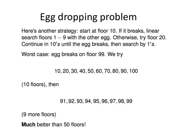
Egg dropping problem
Egg dropping problem
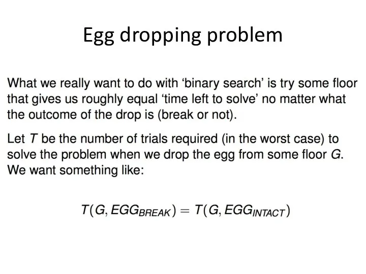
Egg dropping problem
Egg dropping problem
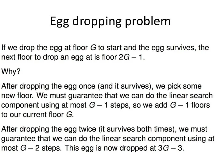
Egg dropping problem
Egg dropping problem
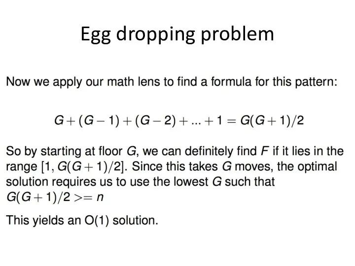
Egg dropping problem
Egg dropping problem
![Egg dropping problem(n eggs) Dynamic Programming Approach D[j,m] : There](/_ipx/f_webp&q_80&fit_contain&s_1440x1080/imagesDir/jpg/598664/slide-35.jpg)
Egg dropping problem(n eggs)
Dynamic Programming Approach
D[j,m] : There are j floors
Egg dropping problem(n eggs)
Dynamic Programming Approach
D[j,m] : There are j floors
![Egg dropping problem(n eggs) Dynamic Programming Approach DP[j,m] : There](/_ipx/f_webp&q_80&fit_contain&s_1440x1080/imagesDir/jpg/598664/slide-36.jpg)
Egg dropping problem(n eggs)
Dynamic Programming Approach
DP[j,m] : There are j floors
Egg dropping problem(n eggs)
Dynamic Programming Approach
DP[j,m] : There are j floors
![Egg dropping problem(n eggs) Dynamic Programming Approach DP[j,m] : There](/_ipx/f_webp&q_80&fit_contain&s_1440x1080/imagesDir/jpg/598664/slide-37.jpg)
Egg dropping problem(n eggs)
Dynamic Programming Approach
DP[j,m] : There are j floors
Egg dropping problem(n eggs)
Dynamic Programming Approach
DP[j,m] : There are j floors
Coin-change Problem
To find the minimum number of Canadian coins to make
Coin-change Problem
To find the minimum number of Canadian coins to make
Coin-change Problem
The greedy method doesn’t work if we didn’t have 5¢
Coin-change Problem
The greedy method doesn’t work if we didn’t have 5¢
Coin set for examples
For the following examples, we will assume coins
Coin set for examples
For the following examples, we will assume coins
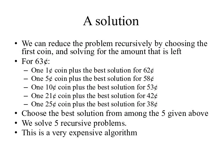
A solution
We can reduce the problem recursively by choosing the first
A solution
We can reduce the problem recursively by choosing the first
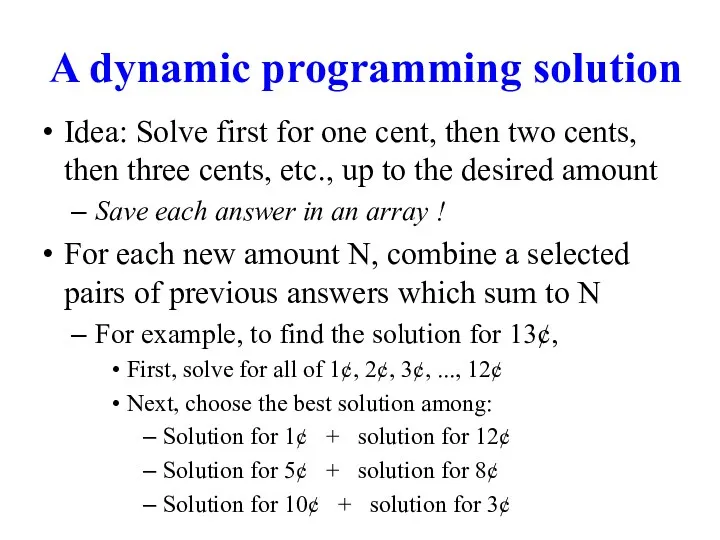
A dynamic programming solution
Idea: Solve first for one cent, then two
A dynamic programming solution
Idea: Solve first for one cent, then two
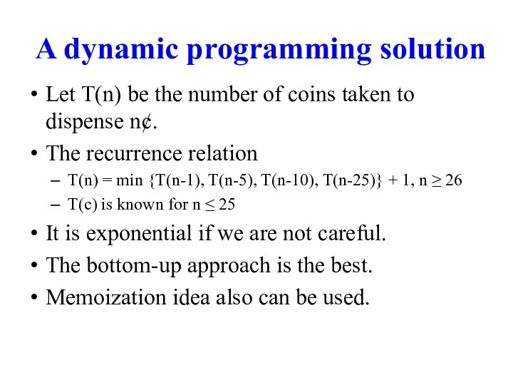
A dynamic programming solution
Let T(n) be the number of coins taken
A dynamic programming solution
Let T(n) be the number of coins taken
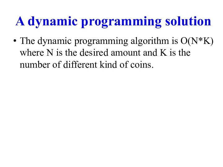
A dynamic programming solution
The dynamic programming algorithm is O(N*K) where N
A dynamic programming solution
The dynamic programming algorithm is O(N*K) where N
Comparison with divide-and-conquer
Divide-and-conquer algorithms split a problem into separate subproblems, solve
Comparison with divide-and-conquer
Divide-and-conquer algorithms split a problem into separate subproblems, solve
Comparison with divide-and-conquer
In contrast, a dynamic programming algorithm proceeds by solving
Comparison with divide-and-conquer
In contrast, a dynamic programming algorithm proceeds by solving
The principle of optimality, I
Dynamic programming is a technique for finding
The principle of optimality, I
Dynamic programming is a technique for finding
The principle of optimality, I
Example: Consider the problem of making N¢
The principle of optimality, I
Example: Consider the problem of making N¢
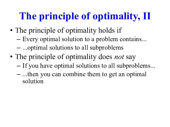
The principle of optimality, II
The principle of optimality holds if
Every optimal
The principle of optimality, II
The principle of optimality holds if
Every optimal
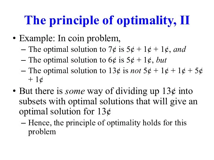
The principle of optimality, II
Example: In coin problem,
The optimal solution to
The principle of optimality, II
Example: In coin problem,
The optimal solution to
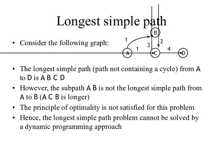
Longest simple path
Consider the following graph:
The longest simple path (path not
Longest simple path
Consider the following graph:
The longest simple path (path not
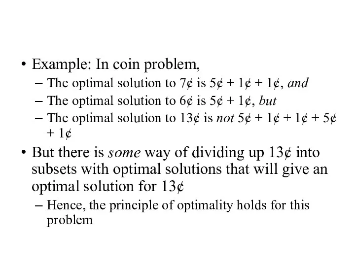
Example: In coin problem,
The optimal solution to 7¢ is 5¢ +
Example: In coin problem,
The optimal solution to 7¢ is 5¢ +
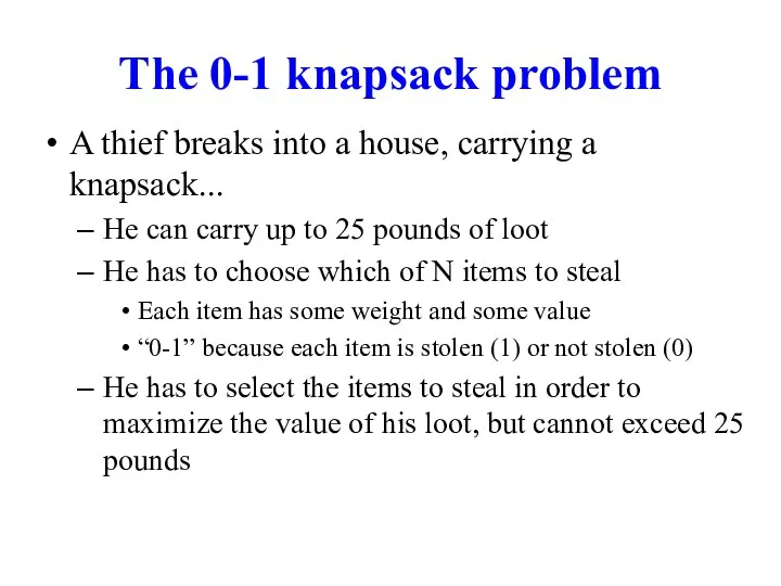
The 0-1 knapsack problem
A thief breaks into a house, carrying a
The 0-1 knapsack problem
A thief breaks into a house, carrying a
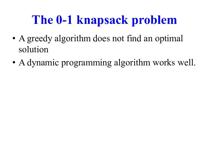
The 0-1 knapsack problem
A greedy algorithm does not find an optimal
The 0-1 knapsack problem
A greedy algorithm does not find an optimal
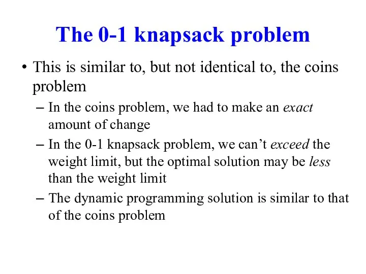
The 0-1 knapsack problem
This is similar to, but not identical to,
The 0-1 knapsack problem
This is similar to, but not identical to,
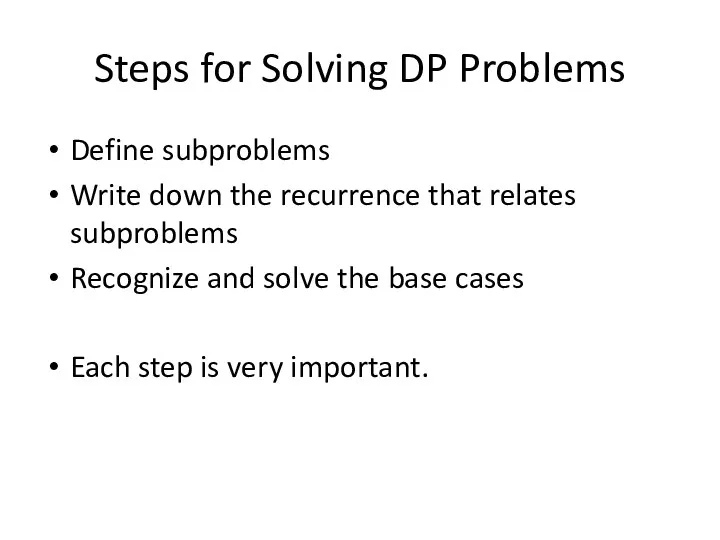
Steps for Solving DP Problems
Define subproblems
Write down the recurrence that relates
Steps for Solving DP Problems
Define subproblems
Write down the recurrence that relates
Comments
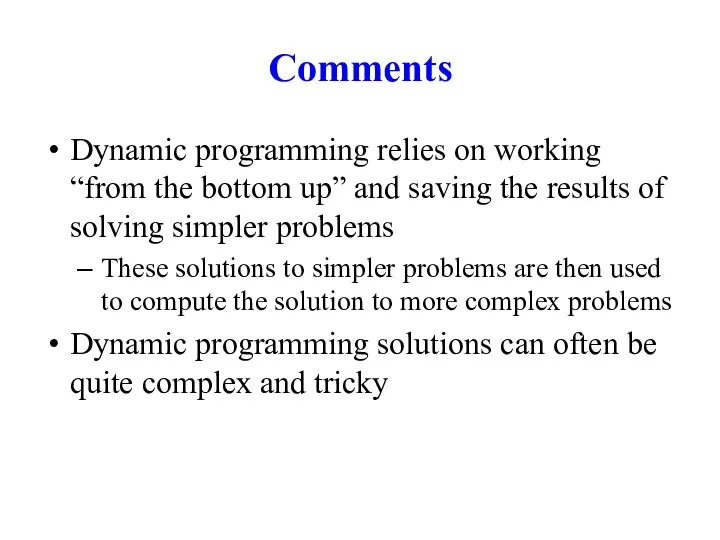
Dynamic programming relies on working “from the bottom up” and saving
Comments
Dynamic programming relies on working “from the bottom up” and saving
 Текстовая информация
 использование игр на уроке информатики в начальной школе
 Spatial Data Structures
 Применение ИКТ на уроках музыки
 Людина у світі інформації
 Организация вычислений в электронных таблицах. Обработка числовой информации в электронных таблицах. Информатика. 9 класс
 Презентация Решение олимпиадных задач. Игра Баше
 Социальные сети для бизнеса
 Testing Throughout the Software Life Cycle: Test Levels. Types of Software Testing (Topic 4)
 Включение системы. Настройка и контроль системы перед отправлением
 Онлайн-кассы
 Шаблоны параллельного проектирования
 9 класс Презентации к урокам
 Управление данными
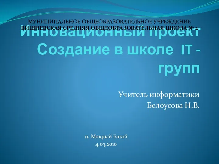 Инновационный проект
 Основы логики.
 Общие и отличительные свойства объектов
 Основы теории коммуникации
 Киберспорт - это спорт?
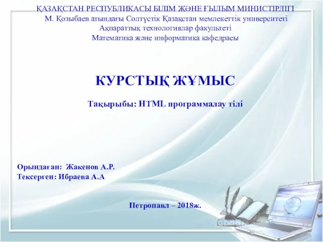 HTML программалау тілі
 Графический редактор Paint
 Объекты JavaScript
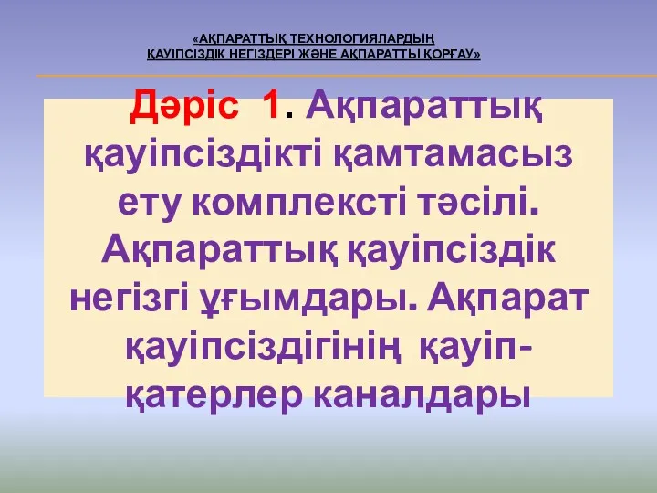 Ақпараттық қауіпсіздікті қамтамасыз ету комплексті тәсілі. Ақпараттық қауіпсіздік негізгі ұғымдары
 Формализация понятия алгоритма
 Культура использования информации. Библиографическое оформление результатов поиска информации
 Solid - принципы с примерами PHP
 Организация интернет-СМИ
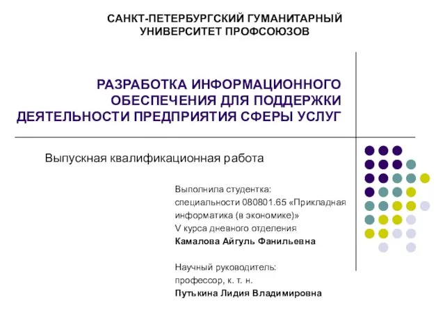 Разработка информационного обеспечения для поддержки деятельности предприятия сферы услуг