- Introduce to Petri nets

Содержание
- 2. Plan Introduction to Petri nets Formal definitions Petri net models of manufacturing system Elementary classes of
- 3. Introduction to Petri nets
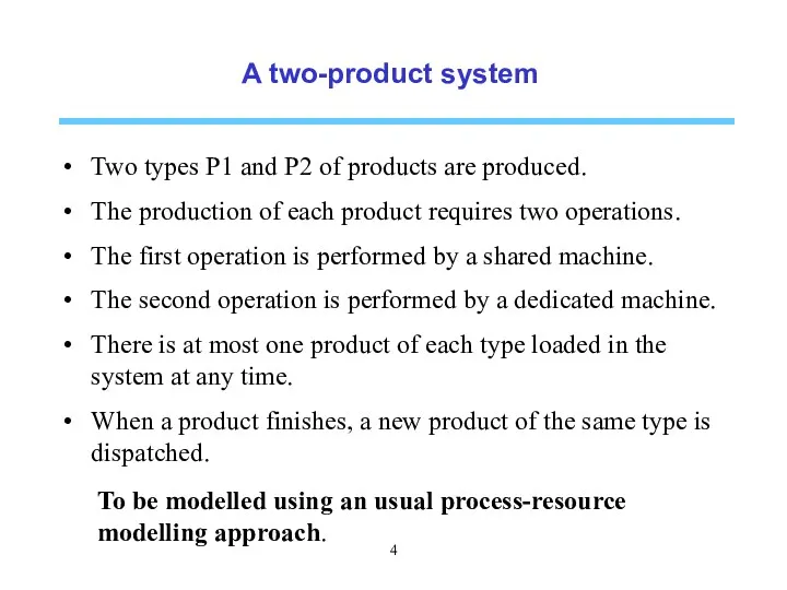
- 4. A two-product system Two types P1 and P2 of products are produced. The production of each
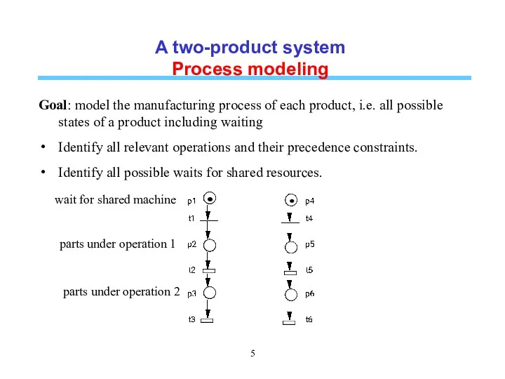
- 5. A two-product system Process modeling Goal: model the manufacturing process of each product, i.e. all possible
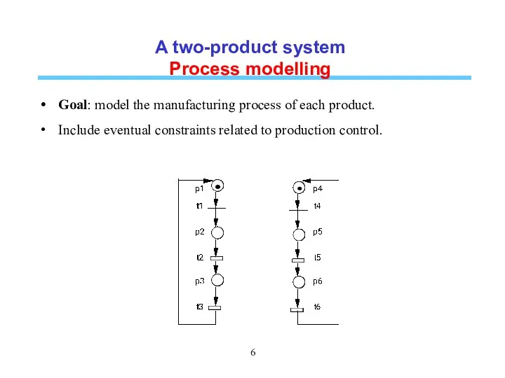
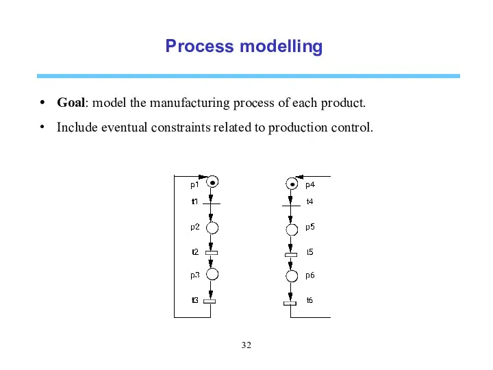
- 6. A two-product system Process modelling Goal: model the manufacturing process of each product. Include eventual constraints
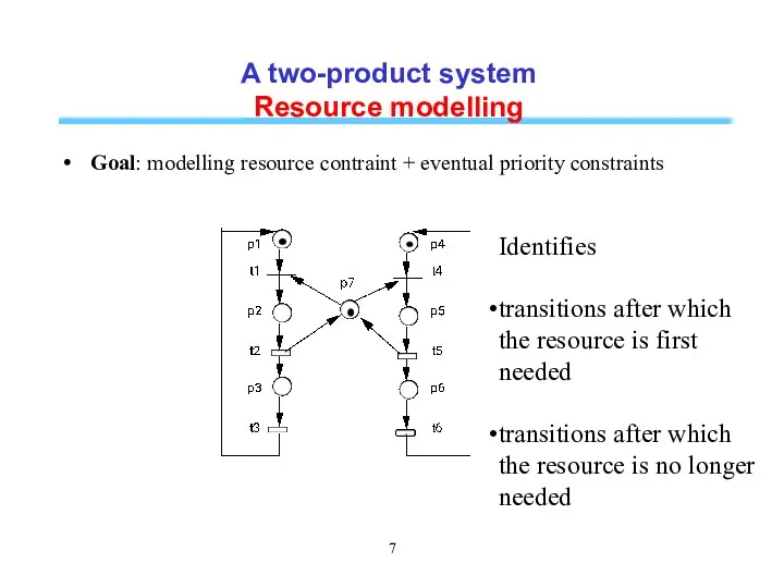
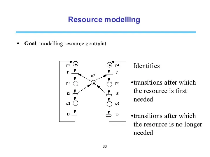
- 7. A two-product system Resource modelling Goal: modelling resource contraint + eventual priority constraints Identifies transitions after
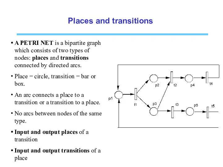
- 8. Places and transitions A PETRI NET is a bipartite graph which consists of two types of
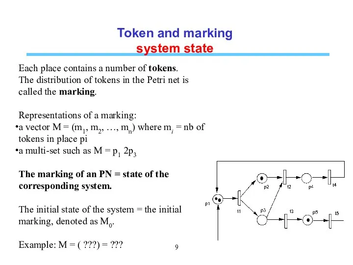
- 9. Token and marking system state Each place contains a number of tokens. The distribution of tokens
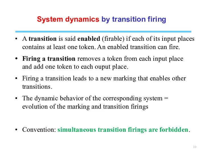
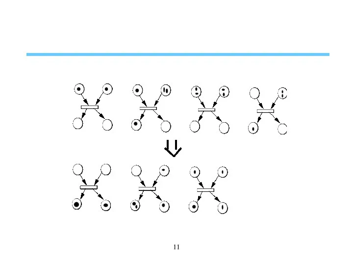
- 10. System dynamics by transition firing A transition is said enabled (firable) if each of its input
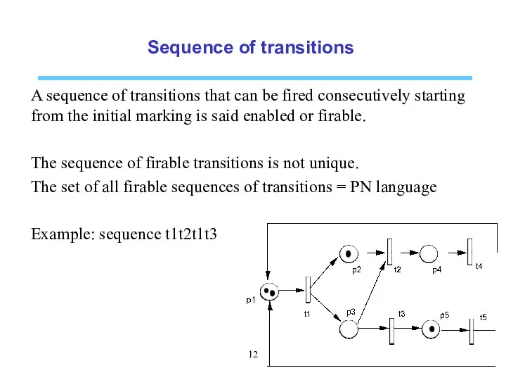
- 12. Sequence of transitions A sequence of transitions that can be fired consecutively starting from the initial
- 13. Formal definitions
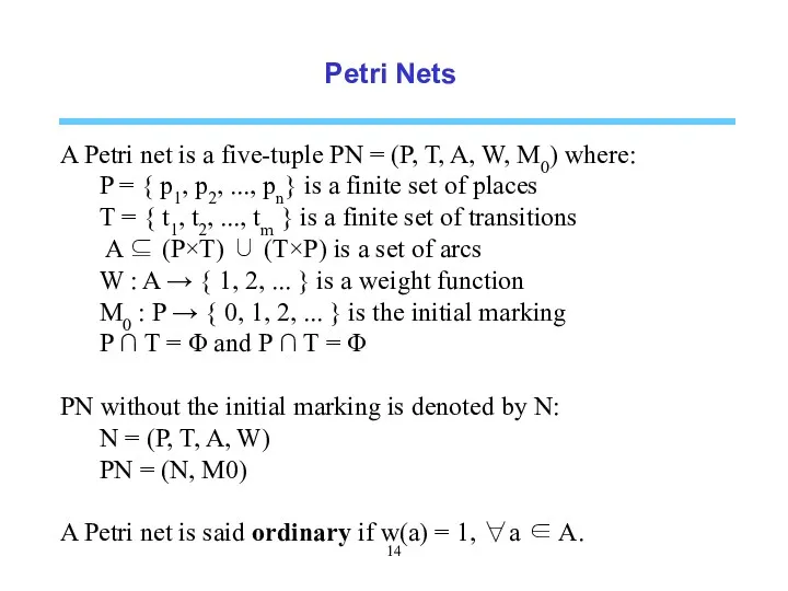
- 14. Petri Nets A Petri net is a five-tuple PN = (P, T, A, W, M0) where:
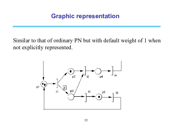
- 15. Graphic representation Similar to that of ordinary PN but with default weight of 1 when not
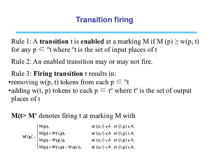
- 16. Transition firing Rule 1: A transition t is enabled at a marking M if M (p)
- 17. Transition firing
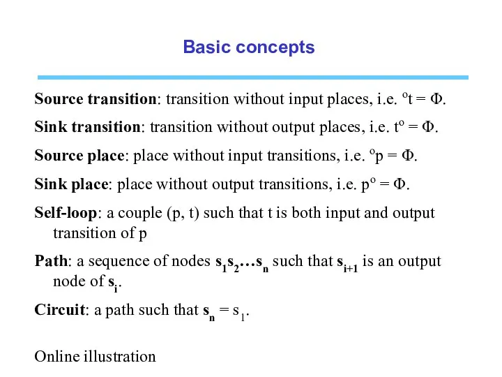
- 18. Basic concepts Source transition: transition without input places, i.e. ot = Φ. Sink transition: transition without
- 19. Incidence matrices Pre incidence matrix: Post incidence matrix: Incidence matrix : C = Post – Pre.
- 20. Incidence matrices Example: Pre = ???, Post = ???, C = ???
- 21. Incidence matrices Enabled transition: A transition t is enabled at a marking M if M ≥
- 22. Incidence matrices Example: Markings after σ = t1t5t2t3t5
- 23. Petri net models of manufacturing systems
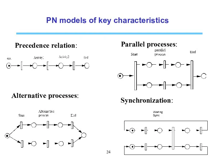
- 24. PN models of key characteristics Precedence relation: Alternative processes: Parallel processes: Synchronization:
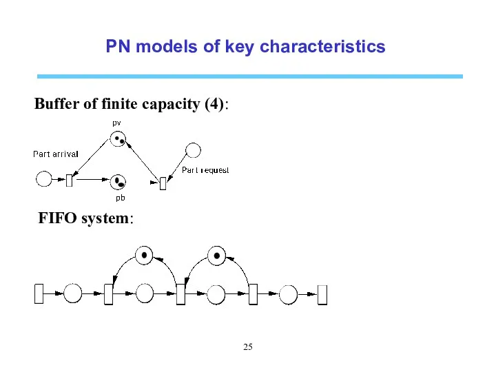
- 25. PN models of key characteristics Buffer of finite capacity (4): FIFO system:
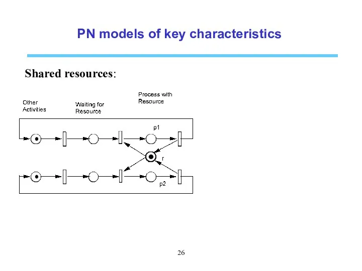
- 26. PN models of key characteristics Shared resources:
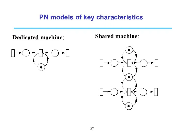
- 27. PN models of key characteristics Dedicated machine: Shared machine:
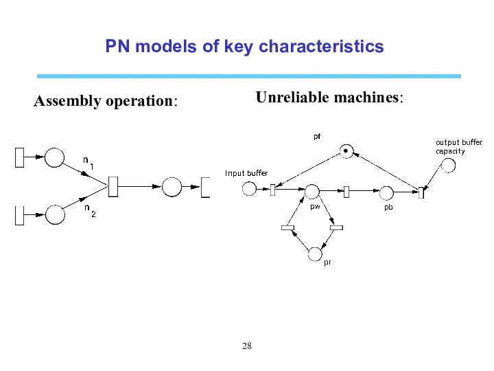
- 28. PN models of key characteristics Assembly operation: Unreliable machines:
- 29. A robotic cell
- 30. A two-product system Two types P1 and P2 of products are produced. The production of each
- 31. Process modeling Goal: model the manufacturing process of each product. Identify all relevant operations and their
- 32. Process modelling Goal: model the manufacturing process of each product. Include eventual constraints related to production
- 33. Resource modelling Goal: modelling resource contraint. Identifies transitions after which the resource is first needed transitions
- 34. Elementary classes of Petri nets
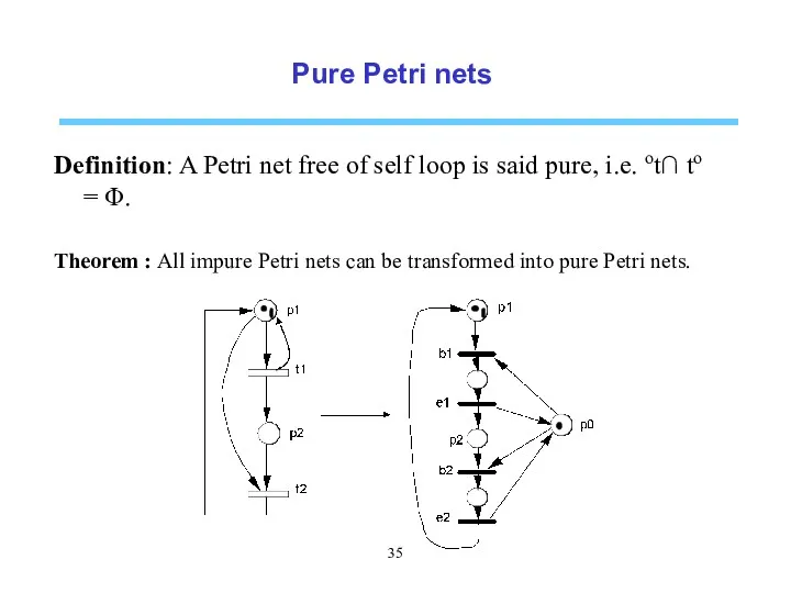
- 35. Pure Petri nets Definition: A Petri net free of self loop is said pure, i.e. ot∩
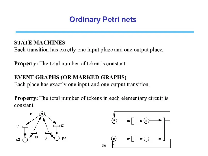
- 36. Ordinary Petri nets STATE MACHINES Each transition has exactly one input place and one output place.
- 37. Ordinary Petri nets FREE-CHOICE NETS card(p°) > 1 ⇒ °(p°) = {p}, ∀ p ∈ P.
- 38. Ordinary Petri nets ASYMMETRIC CHOICE NETS p1°∩p2° ≠ Φ ⇒ p1° ⊆ p2° or p2° ⊆
- 39. Relations between different classes PN = Petri Net AC = Assymmetric choice EFC = Extended Free
- 40. Properties of PN models
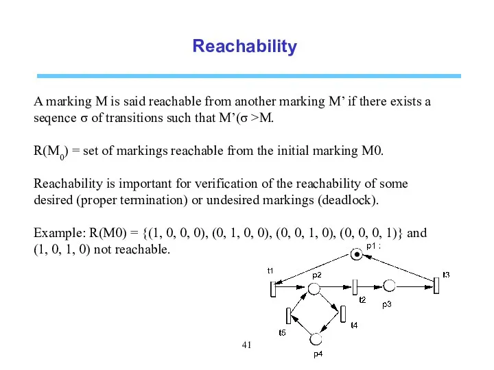
- 41. Reachability A marking M is said reachable from another marking M’ if there exists a seqence
- 42. Reachability Theorem1 (monotonicity) : Any sequence s of transitions firable starting from a marking M0 is
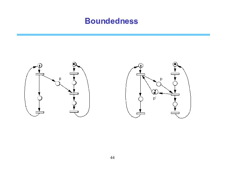
- 43. Boundedness A place p is said k-bounded if the number of tokens in p never exceed
- 44. Boundedness
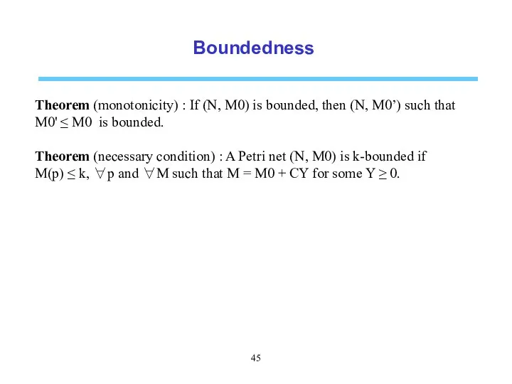
- 45. Boundedness Theorem (monotonicity) : If (N, M0) is bounded, then (N, M0’) such that M0' ≤
- 46. Liveness A transition t is said live if it can always be made enabled starting from
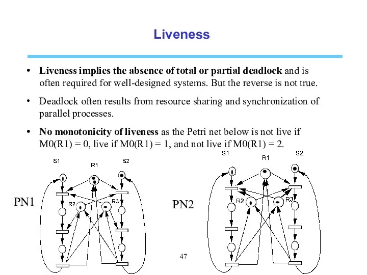
- 47. Liveness Liveness implies the absence of total or partial deadlock and is often required for well-designed
- 48. Reversibility A Petri net (N, M0) is said reversible if the initial marking remains reachable from
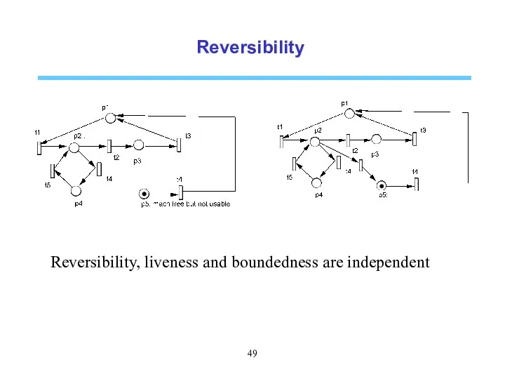
- 49. Reversibility Reversibility, liveness and boundedness are independent
- 50. Analysis methods
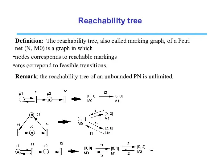
- 51. Reachability tree Definition: The reachability tree, also called marking graph, of a Petri net (N, M0)
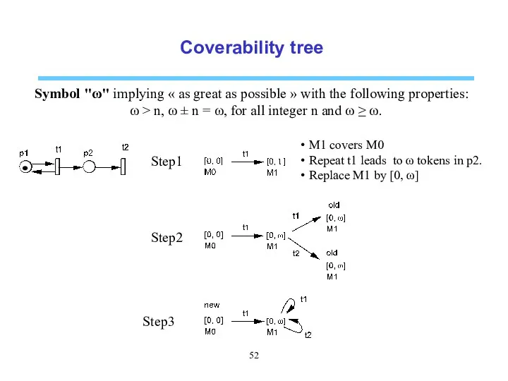
- 52. Coverability tree Symbol "ω" implying « as great as possible » with the following properties: ω
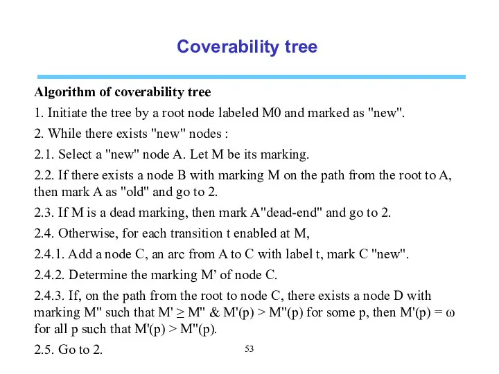
- 53. Coverability tree Algorithm of coverability tree 1. Initiate the tree by a root node labeled M0
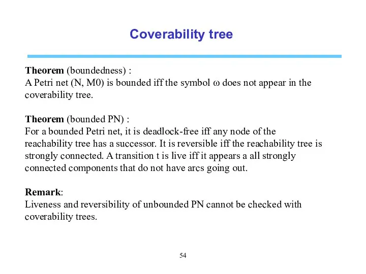
- 54. Coverability tree Theorem (boundedness) : A Petri net (N, M0) is bounded iff the symbol ω
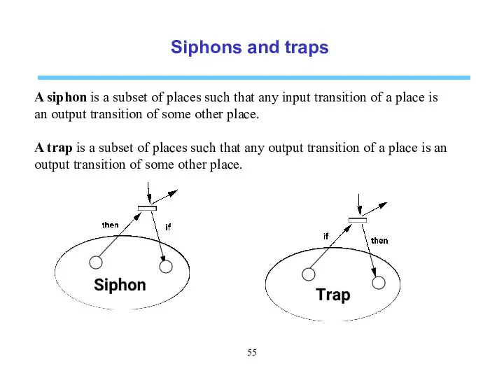
- 55. Siphons and traps A siphon is a subset of places such that any input transition of
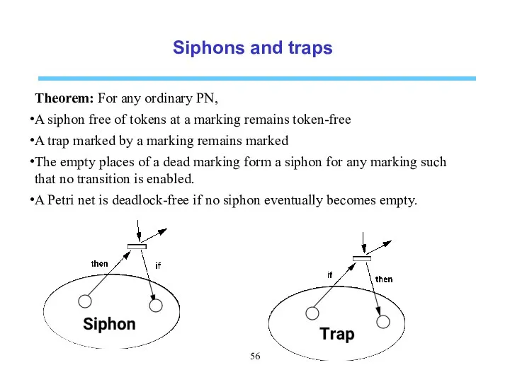
- 56. Siphons and traps Theorem: For any ordinary PN, A siphon free of tokens at a marking
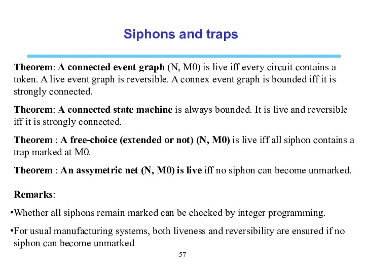
- 57. Siphons and traps Theorem: A connected event graph (N, M0) is live iff every circuit contains
- 58. Siphons and traps Theorem: A Petri net (N, M0) is deadlock-free if G = 0 where
- 59. Siphons and traps Live as it is an AC net and any siphon contain a trap
- 60. p-invariants Definition: A integer vector X≥0 of dimension n = |P| is a p-invariant if Xt
- 61. p-invariants Theorem: X is a p-invariant iff, for all M0, Xt M = Xt M0, ∀
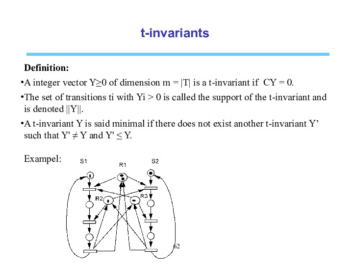
- 62. t-invariants Definition: A integer vector Y≥0 of dimension m = |T| is a t-invariant if CY
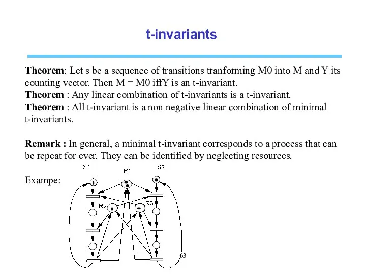
- 63. t-invariants Theorem: Let s be a sequence of transitions tranforming M0 into M and Y its
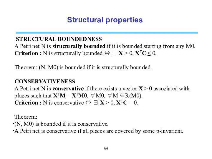
- 64. Structural properties STRUCTURAL BOUNDEDNESS A Petri net N is structurally bounded if it is bounded starting
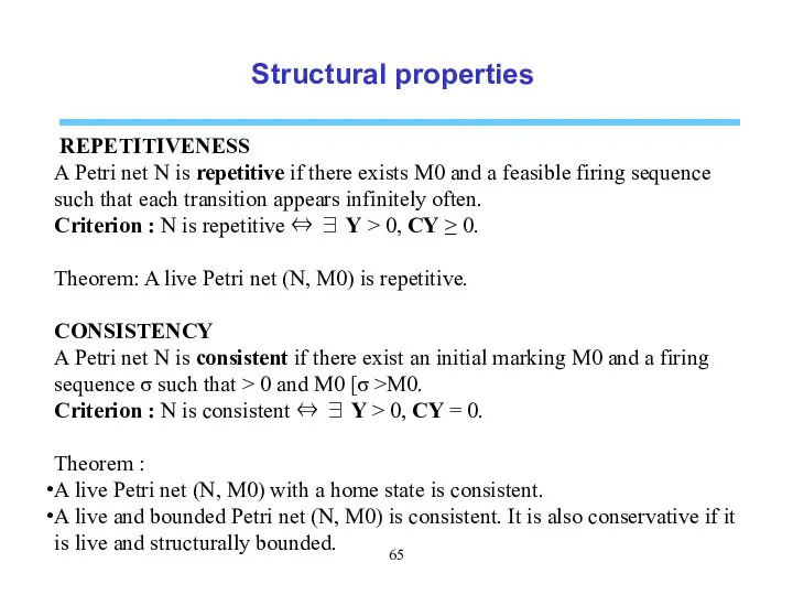
- 65. Structural properties REPETITIVENESS A Petri net N is repetitive if there exists M0 and a feasible
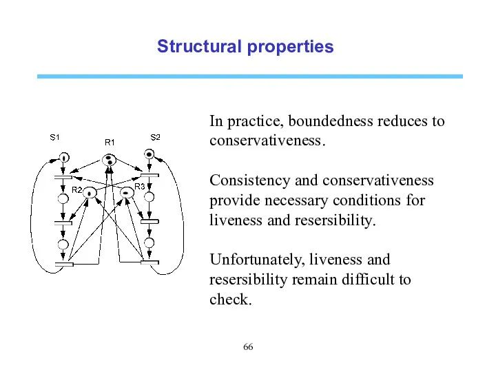
- 66. Structural properties In practice, boundedness reduces to conservativeness. Consistency and conservativeness provide necessary conditions for liveness
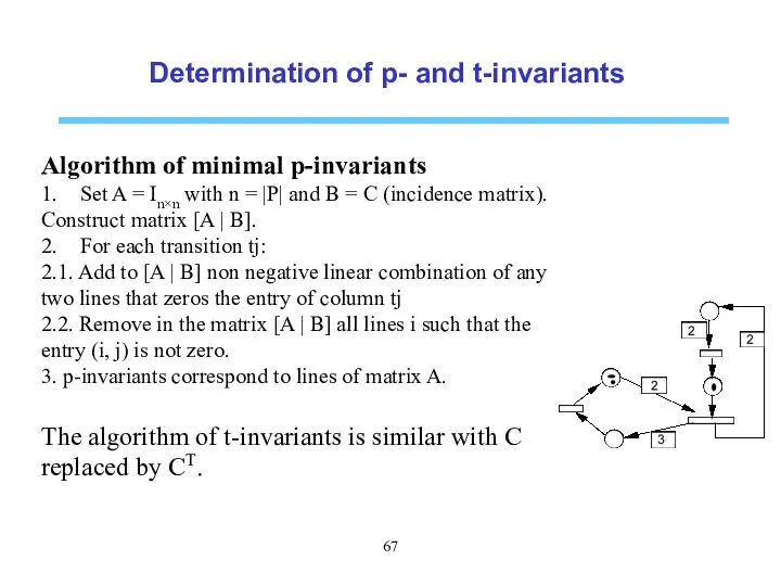
- 67. Determination of p- and t-invariants Algorithm of minimal p-invariants 1. Set A = In×n with n
- 69. Скачать презентацию
Plan
Introduction to Petri nets
Formal definitions
Petri net models of manufacturing system
Elementary classes
Plan
Introduction to Petri nets
Formal definitions
Petri net models of manufacturing system
Elementary classes
Introduction to Petri nets
Introduction to Petri nets
A two-product system
Two types P1 and P2 of products are produced.
The
A two-product system
Two types P1 and P2 of products are produced.
The
A two-product system
Process modeling
Goal: model the manufacturing process of each product,
A two-product system
Process modeling
Goal: model the manufacturing process of each product,
A two-product system
Process modelling
Goal: model the manufacturing process of each product.
Include
A two-product system
Process modelling
Goal: model the manufacturing process of each product.
Include
A two-product system
Resource modelling
Goal: modelling resource contraint + eventual priority constraints
A two-product system
Resource modelling
Goal: modelling resource contraint + eventual priority constraints
Places and transitions
A PETRI NET is a bipartite graph which consists
Places and transitions
A PETRI NET is a bipartite graph which consists
Token and marking
system state
Each place contains a number of tokens.
The
Token and marking
system state
Each place contains a number of tokens.
The
System dynamics by transition firing
A transition is said enabled (firable) if
System dynamics by transition firing
A transition is said enabled (firable) if
Sequence of transitions
A sequence of transitions that can be fired consecutively
Sequence of transitions
A sequence of transitions that can be fired consecutively

Formal definitions
Formal definitions
Petri Nets
A Petri net is a five-tuple PN = (P, T,
Petri Nets
A Petri net is a five-tuple PN = (P, T,
Graphic representation
Similar to that of ordinary PN but with default weight
Graphic representation
Similar to that of ordinary PN but with default weight
Transition firing
Rule 1: A transition t is enabled at a marking
Transition firing
Rule 1: A transition t is enabled at a marking
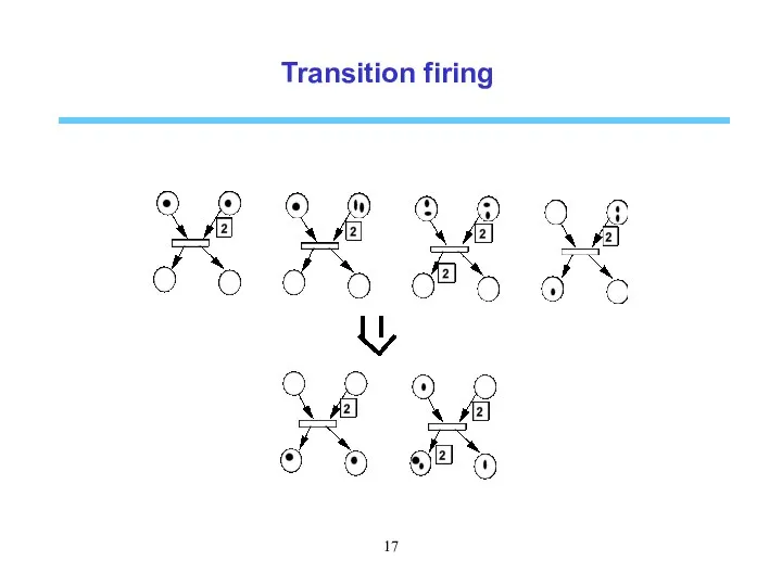
Transition firing
Transition firing
Basic concepts
Source transition: transition without input places, i.e. ot = Φ.
Sink
Basic concepts
Source transition: transition without input places, i.e. ot = Φ.
Sink
Incidence matrices
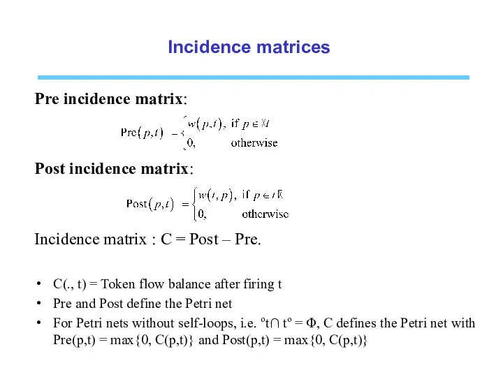
Pre incidence matrix:
Post incidence matrix:
Incidence matrix : C = Post
Incidence matrices
Pre incidence matrix:
Post incidence matrix:
Incidence matrix : C = Post
Incidence matrices
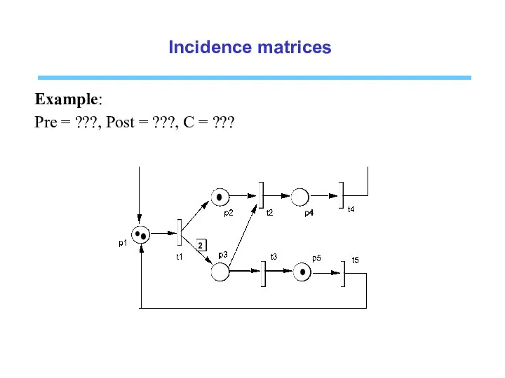
Example:
Pre = ???, Post = ???, C = ???
Incidence matrices
Example:
Pre = ???, Post = ???, C = ???
Incidence matrices
Enabled transition: A transition t is enabled at a marking
Incidence matrices
Enabled transition: A transition t is enabled at a marking
Incidence matrices
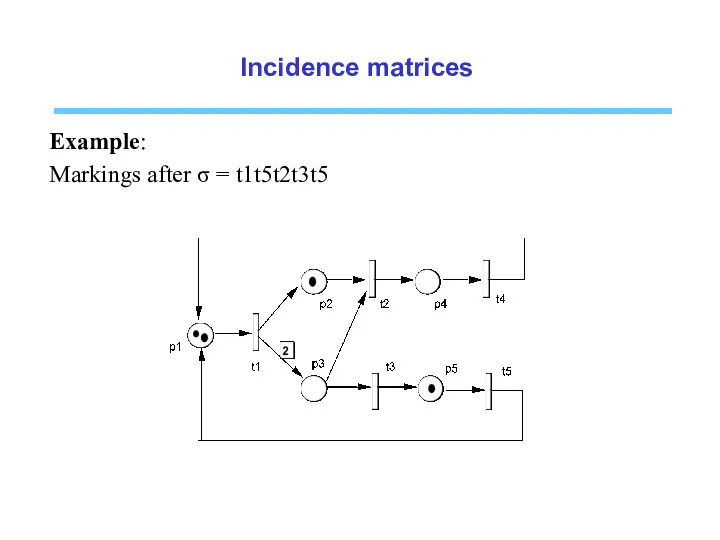
Example:
Markings after σ = t1t5t2t3t5
Incidence matrices
Example:
Markings after σ = t1t5t2t3t5
Petri net models of manufacturing systems
Petri net models of manufacturing systems
PN models of key characteristics
Precedence relation:
Alternative processes:
Parallel processes:
Synchronization:
PN models of key characteristics
Precedence relation:
Alternative processes:
Parallel processes:
Synchronization:
PN models of key characteristics
Buffer of finite capacity (4):
FIFO system:
PN models of key characteristics
Buffer of finite capacity (4):
FIFO system:
PN models of key characteristics
Shared resources:
PN models of key characteristics
Shared resources:
PN models of key characteristics
Dedicated machine:
Shared machine:
PN models of key characteristics
Dedicated machine:
Shared machine:
PN models of key characteristics
Assembly operation:
Unreliable machines:
PN models of key characteristics
Assembly operation:
Unreliable machines:
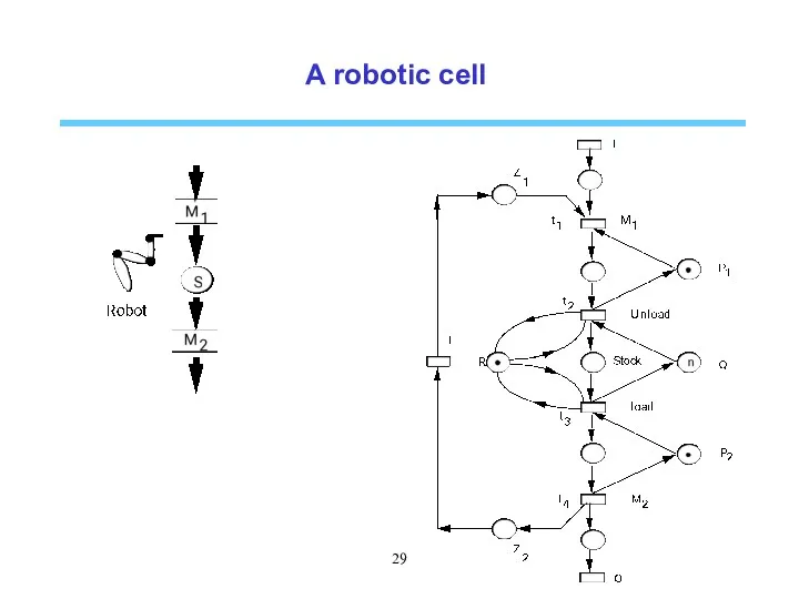
A robotic cell
A robotic cell

A two-product system
Two types P1 and P2 of products are produced.
The
A two-product system
Two types P1 and P2 of products are produced.
The
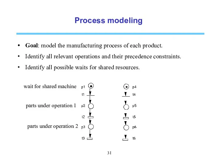
Process modeling
Goal: model the manufacturing process of each product.
Identify all relevant
Process modeling
Goal: model the manufacturing process of each product.
Identify all relevant
Process modelling
Goal: model the manufacturing process of each product.
Include eventual constraints
Process modelling
Goal: model the manufacturing process of each product.
Include eventual constraints
Resource modelling
Goal: modelling resource contraint.
Identifies
transitions after which the resource is
Resource modelling
Goal: modelling resource contraint.
Identifies
transitions after which the resource is

Elementary classes of Petri nets
Elementary classes of Petri nets
Pure Petri nets
Definition: A Petri net free of self loop is
Pure Petri nets
Definition: A Petri net free of self loop is
Ordinary Petri nets
STATE MACHINES
Each transition has exactly one input place and
Ordinary Petri nets
STATE MACHINES
Each transition has exactly one input place and
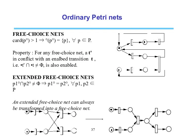
Ordinary Petri nets
FREE-CHOICE NETS
card(p°) > 1 ⇒ °(p°) = {p}, ∀
Ordinary Petri nets
FREE-CHOICE NETS
card(p°) > 1 ⇒ °(p°) = {p}, ∀
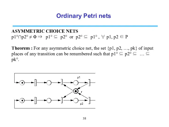
Ordinary Petri nets
ASYMMETRIC CHOICE NETS
p1°∩p2° ≠ Φ ⇒ p1° ⊆ p2°
Ordinary Petri nets
ASYMMETRIC CHOICE NETS
p1°∩p2° ≠ Φ ⇒ p1° ⊆ p2°
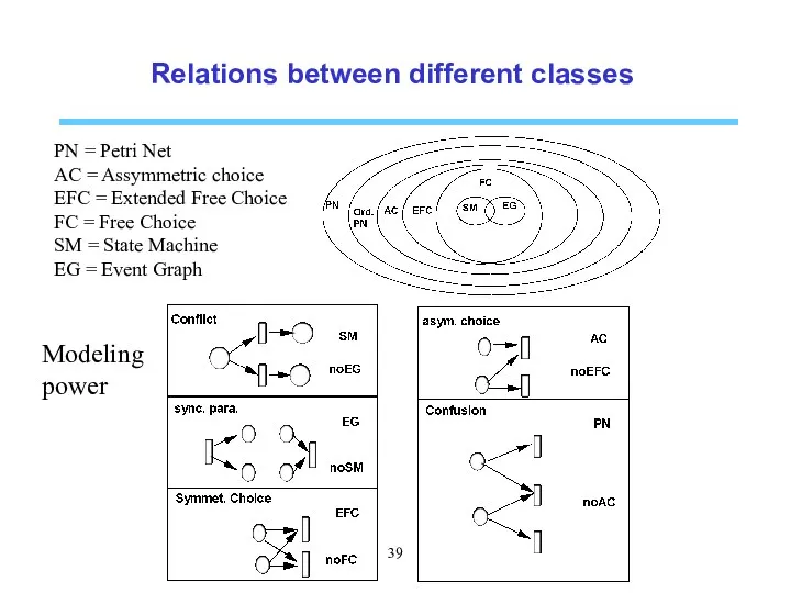
Relations between different classes
PN = Petri Net
AC = Assymmetric choice
EFC =
Relations between different classes
PN = Petri Net
AC = Assymmetric choice
EFC =
Properties of PN models
Properties of PN models
Reachability
A marking M is said reachable from another marking M’ if
Reachability
A marking M is said reachable from another marking M’ if
Reachability
Theorem1 (monotonicity) : Any sequence s of transitions firable starting from
Reachability
Theorem1 (monotonicity) : Any sequence s of transitions firable starting from
Boundedness
A place p is said k-bounded if the number of tokens
Boundedness
A place p is said k-bounded if the number of tokens
Boundedness
Boundedness
Boundedness
Theorem (monotonicity) : If (N, M0) is bounded, then (N, M0’)
Boundedness
Theorem (monotonicity) : If (N, M0) is bounded, then (N, M0’)

Liveness
A transition t is said live if it can always be
Liveness
A transition t is said live if it can always be
Liveness
Liveness implies the absence of total or partial deadlock and is
Liveness
Liveness implies the absence of total or partial deadlock and is
Reversibility
A Petri net (N, M0) is said reversible if the initial
Reversibility
A Petri net (N, M0) is said reversible if the initial
Reversibility
Reversibility, liveness and boundedness are independent
Reversibility
Reversibility, liveness and boundedness are independent
Analysis methods
Analysis methods
Reachability tree
Definition: The reachability tree, also called marking graph, of a
Reachability tree
Definition: The reachability tree, also called marking graph, of a
Coverability tree
Symbol "ω" implying « as great as possible » with the following
Coverability tree
Symbol "ω" implying « as great as possible » with the following
Coverability tree
Algorithm of coverability tree
1. Initiate the tree by a root
Coverability tree
Algorithm of coverability tree
1. Initiate the tree by a root
Coverability tree
Theorem (boundedness) :
A Petri net (N, M0) is bounded
Coverability tree
Theorem (boundedness) :
A Petri net (N, M0) is bounded
Siphons and traps
A siphon is a subset of places such that
Siphons and traps
A siphon is a subset of places such that
Siphons and traps
Theorem: For any ordinary PN,
A siphon free of tokens
Siphons and traps
Theorem: For any ordinary PN,
A siphon free of tokens
Siphons and traps
Theorem: A connected event graph (N, M0) is live
Siphons and traps
Theorem: A connected event graph (N, M0) is live
Siphons and traps
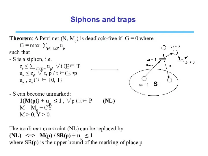
Theorem: A Petri net (N, M0) is deadlock-free if
Siphons and traps
Theorem: A Petri net (N, M0) is deadlock-free if
Siphons and traps
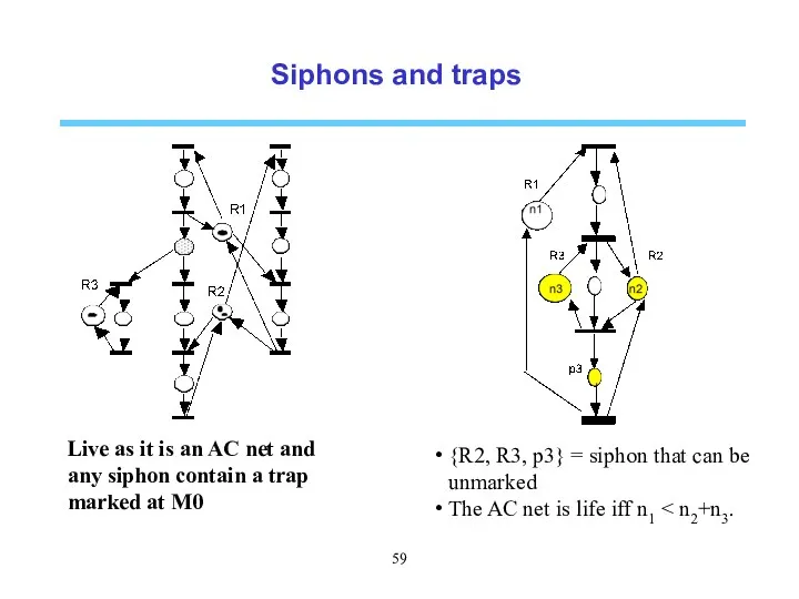
Live as it is an AC net and any
Siphons and traps
Live as it is an AC net and any
p-invariants
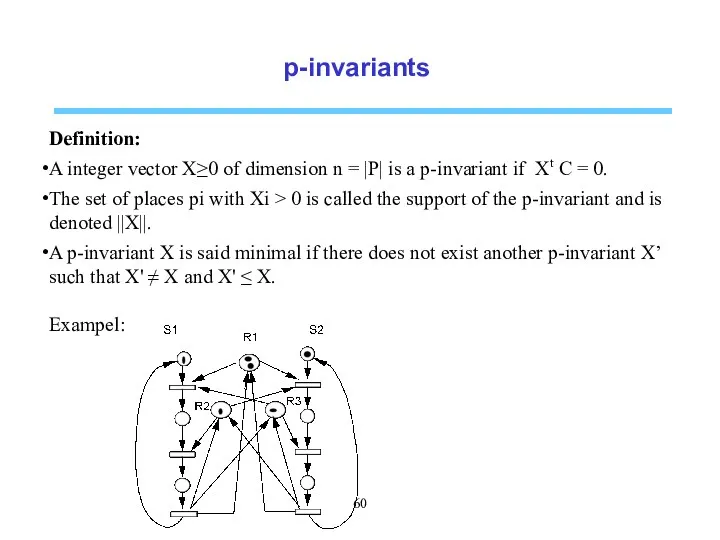
Definition:
A integer vector X≥0 of dimension n = |P| is
p-invariants
Definition:
A integer vector X≥0 of dimension n = |P| is
p-invariants
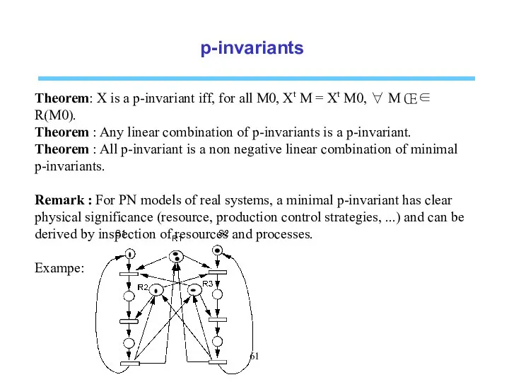
Theorem: X is a p-invariant iff, for all M0, Xt M
p-invariants
Theorem: X is a p-invariant iff, for all M0, Xt M
t-invariants
Definition:
A integer vector Y≥0 of dimension m = |T| is
t-invariants
Definition:
A integer vector Y≥0 of dimension m = |T| is
t-invariants
Theorem: Let s be a sequence of transitions tranforming M0 into
t-invariants
Theorem: Let s be a sequence of transitions tranforming M0 into
Structural properties
STRUCTURAL BOUNDEDNESS
A Petri net N is structurally bounded
Structural properties
STRUCTURAL BOUNDEDNESS
A Petri net N is structurally bounded
Structural properties
REPETITIVENESS
A Petri net N is repetitive if there exists M0
Structural properties
REPETITIVENESS
A Petri net N is repetitive if there exists M0
Structural properties
In practice, boundedness reduces to conservativeness.
Consistency and conservativeness provide necessary
Structural properties
In practice, boundedness reduces to conservativeness.
Consistency and conservativeness provide necessary
Determination of p- and t-invariants
Algorithm of minimal p-invariants
1. Set A =
Determination of p- and t-invariants
Algorithm of minimal p-invariants
1. Set A =
 Компьютерная графика
 Средства обеспечение компьютерной безопасности. Антивирусные программы
 Сериализация. (Лекция 4)
 Алгоритмы и модели трассировки печатных соединений в ЭС. Лекция 5
 Дистанционное обучение
 Анализ данных в реляционных БД на примере СУБД MS Access
 Microsoft Word Работа с объектами
 Программный продукт АРМ Экспедитор 1015
 Повторение Адрес клетки. Устройства компьютера
 Школьная библиотека: Копилочка. Инновационные формы профессионального взаимодействия
 Устав команды поддержки
 Тармақталу алгоритмдерін программалау
 SOLID (single responsibility, openclosed, Liskov substitution, interface segregation, dependency inversion)
 Основы программирования. Лекция № 2
 Программалау тарихы
 тест Растровая и векторная графика
 Web-программирование
 Информация о платформах дистанционного обучения
 Перегрузка операторов. Лекция 38
 Web-сайт және түрлері
 Поиск информации в базе данных. ОГЭ по информатике, задача 12
 Графические операторы языка Qbasic
 Система самообслуживания клиентов
 Программирование на языке Паскаль
 Одномерные массивы (последовательности)
 Интенсив-курс по React JS
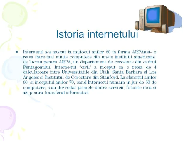 Istoria internetului/
 Методическая разработка урока Знаки и знаковые системы 8 класс