- Modelling and Simulation IS 331. Lec (2)

Содержание
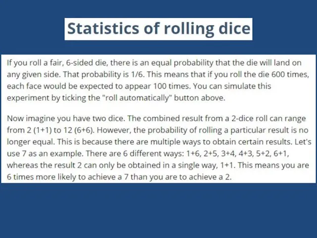
- 2. Recap: Performance Evaluation Performance Evaluation Performance Measurement Analytic Modeling Simulation Performance Modeling
- 3. Simulation Model Taxonomy (preview)
- 4. A system is defined as a group of objects that interact with each other to accomplish
- 5. Entity An object of interest in the system: Machines in factory Attribute The property of an
- 6. When the problem can be solved by common sense When the problem can be solved analytically
- 7. Monte Carlo simulation Time-stepped simulation Trace-driven simulation Discrete-event simulation Continuous simulation Types of Simulations
- 8. Simulation Model Taxonomy
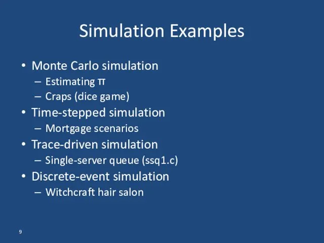
- 9. Monte Carlo simulation Estimating π Craps (dice game) Time-stepped simulation Mortgage scenarios Trace-driven simulation Single-server queue
- 10. Monte Carlo simulation Estimating π Craps (dice game) Simulation Examples
- 11. Static simulation (no time dependency) To model probabilistic phenomenon Can be used for evaluating non-probabilistic expressions
- 12. Classic Example Find the value of ? Use the reject and accept method Or hit and
- 19. Monte Carlo simulation Estimating π Craps (dice game) Simulation Examples
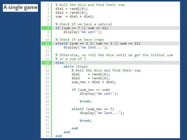
- 20. Monte Carlo Simulation of the Craps Dice Game
- 21. Basics The player rolling the dice is the "shooter". Shooters first throw in a round of
- 22. Objective The basic objective in Craps is for the shooter to win by tossing the Point
- 23. Craps Game
- 24. Questions What is the probability that the roller wins? Note that this is not a simple
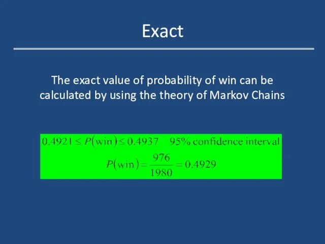
- 27. Exact The exact value of probability of win can be calculated by using the theory of
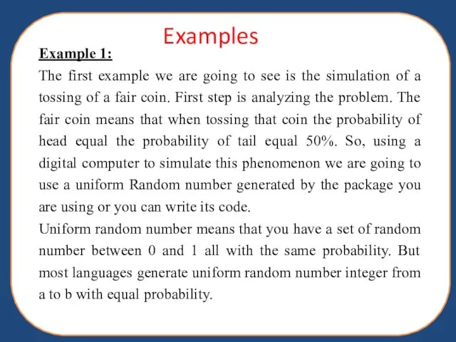
- 28. Examples Example 1: The first example we are going to see is the simulation of a
- 29. See the following program written in c++ #include #include void main(void) { int x,nuber_or_trials, head=0, tail=0;
- 30. The output results are: Enter number of trials = 1 probability of head= 0 with error
- 31. Example2 Get the average daily demand for a small grocery store selling a fresh bread according
- 32. To simulate the daily demand(5 days) Draw one ball at a time, notice its color and
- 34. Скачать презентацию
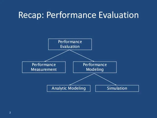
Recap: Performance Evaluation
Performance Evaluation
Performance Measurement
Analytic Modeling
Simulation
Performance Modeling
Recap: Performance Evaluation
Performance Evaluation
Performance Measurement
Analytic Modeling
Simulation
Performance Modeling
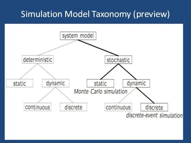
Simulation Model Taxonomy (preview)
Simulation Model Taxonomy (preview)
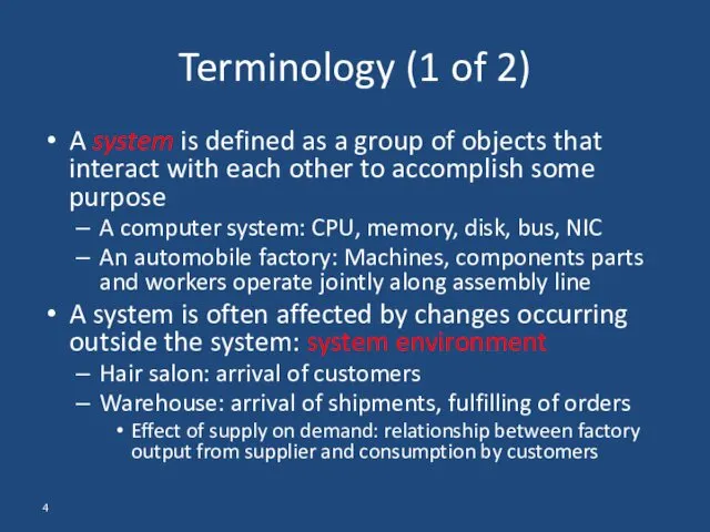
A system is defined as a group of objects that interact
A system is defined as a group of objects that interact
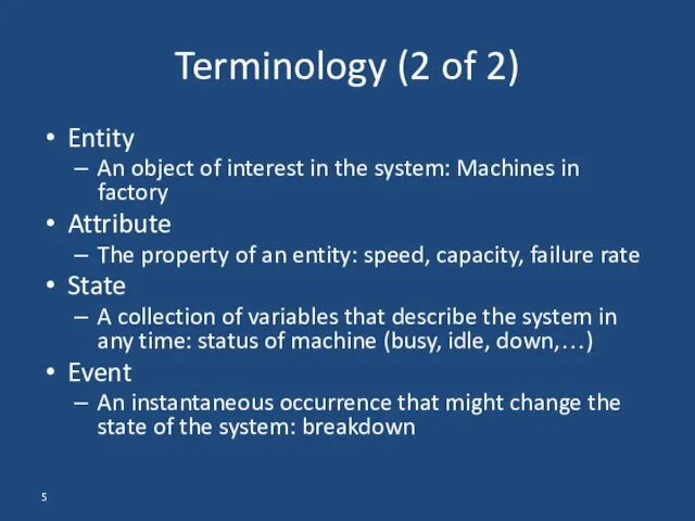
Entity
An object of interest in the system: Machines in factory
Attribute
The property
Entity
An object of interest in the system: Machines in factory
Attribute
The property
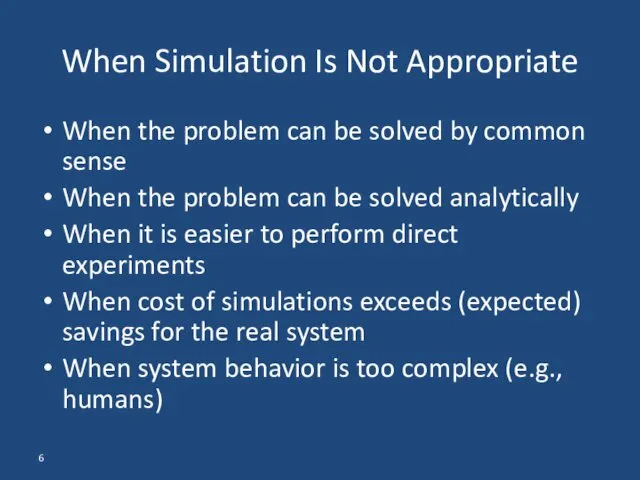
When the problem can be solved by common sense
When the problem
When the problem can be solved by common sense
When the problem
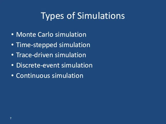
Monte Carlo simulation
Time-stepped simulation
Trace-driven simulation
Discrete-event simulation
Continuous simulation
Types of Simulations
Monte Carlo simulation
Time-stepped simulation
Trace-driven simulation
Discrete-event simulation
Continuous simulation
Types of Simulations
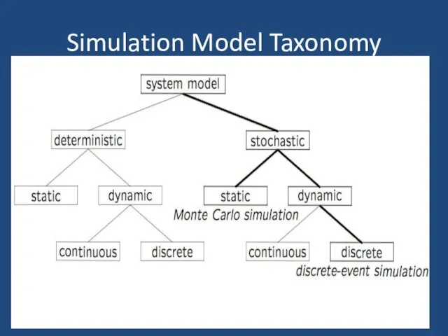
Simulation Model Taxonomy
Simulation Model Taxonomy
Monte Carlo simulation
Estimating π
Craps (dice game)
Time-stepped simulation
Mortgage scenarios
Trace-driven simulation
Single-server queue (ssq1.c)
Discrete-event
Monte Carlo simulation
Estimating π
Craps (dice game)
Time-stepped simulation
Mortgage scenarios
Trace-driven simulation
Single-server queue (ssq1.c)
Discrete-event
Monte Carlo simulation
Estimating π
Craps (dice game)
Simulation Examples
Monte Carlo simulation
Estimating π
Craps (dice game)
Simulation Examples
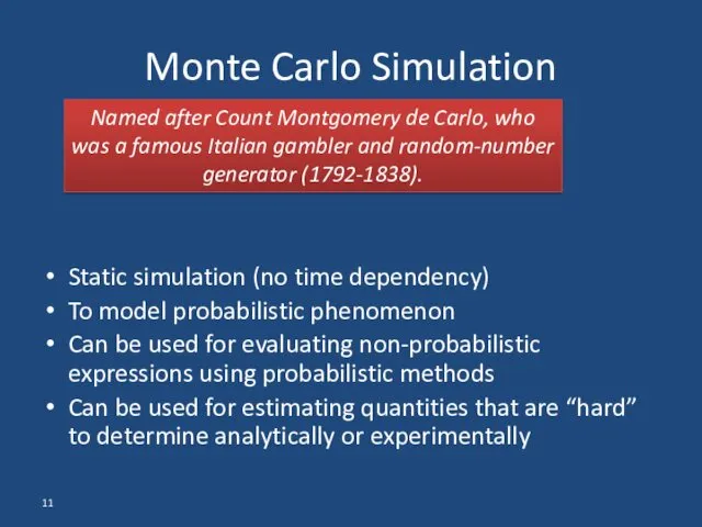
Static simulation (no time dependency)
To model probabilistic phenomenon
Can be used
Static simulation (no time dependency)
To model probabilistic phenomenon
Can be used
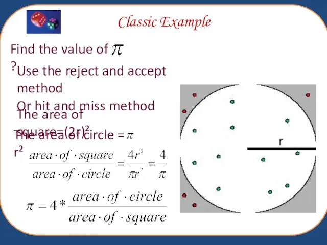
Classic Example
Find the value of ?
Use the reject and accept
Classic Example
Find the value of ?
Use the reject and accept


Monte Carlo simulation
Estimating π
Craps (dice game)
Simulation Examples
Monte Carlo simulation
Estimating π
Craps (dice game)
Simulation Examples
Monte Carlo Simulation
of the Craps Dice Game
Monte Carlo Simulation
of the Craps Dice Game
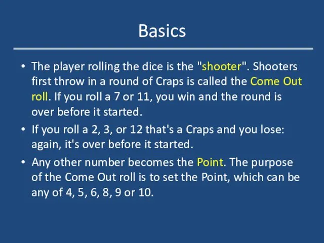
Basics
The player rolling the dice is the "shooter". Shooters first throw
Basics
The player rolling the dice is the "shooter". Shooters first throw
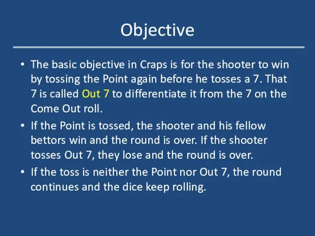
Objective
The basic objective in Craps is for the shooter to win
Objective
The basic objective in Craps is for the shooter to win
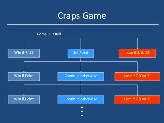
Craps Game
Craps Game
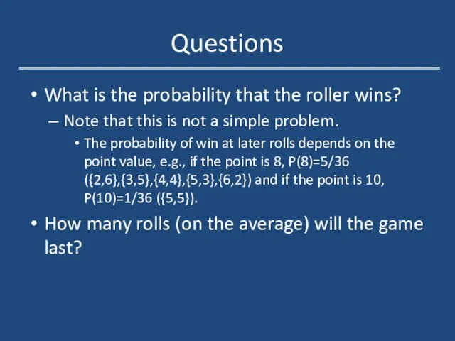
Questions
What is the probability that the roller wins?
Note that this is
Questions
What is the probability that the roller wins?
Note that this is

Exact
The exact value of probability of win can be calculated by
Exact
The exact value of probability of win can be calculated by
Examples
Example 1:
The first example we are going to see is the
Examples
Example 1:
The first example we are going to see is the
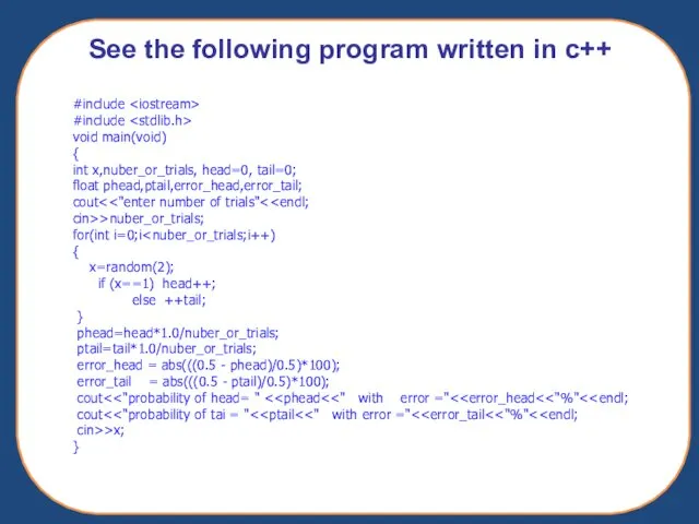
See the following program written in c++
#include
#include
void main(void)
{
int x,nuber_or_trials,
See the following program written in c++
#include
#include
void main(void)
{
int x,nuber_or_trials,
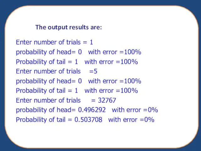
The output results are:
Enter number of trials = 1
probability of head=
The output results are:
Enter number of trials = 1
probability of head=
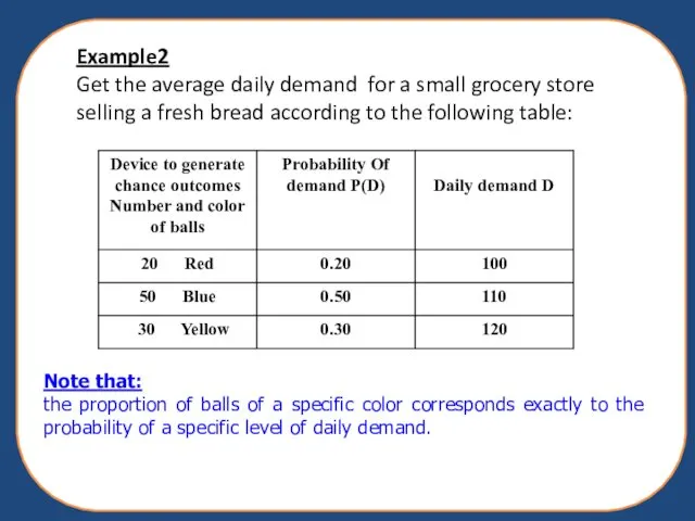
Example2
Get the average daily demand for a small grocery store selling
Example2 Get the average daily demand for a small grocery store selling
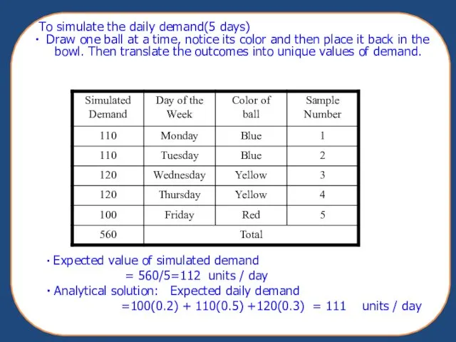
To simulate the daily demand(5 days)
Draw one ball at a
To simulate the daily demand(5 days)
Draw one ball at a
 Программное обеспечение (Software)
 Академия Арктикбота
 Проектирование волоконно-оптической линии связи на железнодорожном участке Лоухи
 Второй уровень информационного взаимодействия. Вторичные информационные процессы
 3D - үлгілерін құру
 Язык программирования общего назначения Python
 Принципы функционирования компьютерных сетей. (Лекция 1)
 HTML document
 XSS Межсайтовый скриптинг
 Компьютерные сети. § 44. Основные понятия. 10 класс
 Виды, цели и уровни интеграции программных модулей
 Информатизация как ресурс повышения качества образования
 Разработка игр на Unity 2021_2022 (методичка)
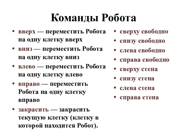 Задание ОГЭ. Команды Робота
 Формат издания
 Как пользоваться пин-падом при обслуживании карт
 Создание мобильной версии сайта
 Разработка урока по теме:Логика
 Кодирование и обработка текстовой информации. Урок – зачет
 Как сделать WiFi в лесу на 500 человек
 3. Essential Java Classes. 3a. Date and Time in Java SE8
 Применение технологии блокчейн
 47320
47320 CSS-препроцесор SASS/SCSS (продовження)
 Браузеры. Яндекс Браузер, Opera, Firefox
 Системы автоматизированного проектирования технологических процессов. Программное обеспечение САПР ТП. (Лекция 3)
 Введение. Основные понятия машинного обучения. Применение машинного обучения в искусственном интеллекте
 Віртуальна реальність