- Neural networks

Содержание
- 2. Table of contents The basic concepts of neural networks Artificial neural networks. The structure of an
- 3. Self-organizing maps The principle of unsupervised learning. Kohonen self-organizing maps. Learning Kohonen networks. Practical using of
- 4. References David Kriesel. A brief Introduction to Neural networks // http://www.dkriesel.com/en/science/neural_networks Raul Rojas. Neural Networks. A
- 5. The basic concepts of neural networks
- 6. Questions for motivation discussion What tasks are machines good at doing that humans are not? What
- 7. Types of learning Knowledge acquisition from expert. Knowledge acquisition from data: Supervised learning – the system
- 8. Artificial Neural Network An extremely simplified model of the human’s brain Transforms inputs into the best
- 9. Artificial Neural Networks Development of Neural Networks date back to the early 1940s. It experienced an
- 10. ANN vs Computers Computers have to be explicitly programmed Analyze the problem to be solved. Write
- 11. ANN vs Computers Digital Computers Deductive Reasoning. We apply known rules to input data to produce
- 12. Biological neuron
- 13. Biological neuron Many “neurons” co-operate to perform the desired function Basic elements: Axon Dendrite Synapse
- 14. Artificial Neuron Structure The output of a neuron is a function of the weighted sum of
- 15. Common activation functions
- 17. Examples of ANN topologies Single layer ANN Multilayer ANN ANN with one recurrent layer
- 18. Fundamentals of learning and training samples The weights in a neural network are the most important
- 19. Fundamentals of learning and training samples There are two main types of training Supervised Training Supplies
- 20. Fundamentals of learning and training samples A training pattern is an input vector p with the
- 21. Fundamentals of learning and training samples Teaching input. Let j be an output neuron. The teaching
- 22. Fundamentals of learning and training samples Error vector. For several output neurons Ω1,Ω2, . . .
- 23. Fundamentals of learning Let P be the set of training patters. In learning procedure we realize
- 24. General learning procedure Let P be the set of n training patters pn For i=1 to
- 25. Using training samples We have to divide the set of training samples into two subsets: one
- 26. Learning curve The learning curve indicates the progress of the error, which can be determined in
- 27. Error measurement Let Ω be the output neuron and O be the set of output neurons.
- 28. When do we stop learning? Generally, the training process is stopped when the user in front
- 29. Using neural networks in practice (discussion) Classification in marketing: consumer spending pattern classification In defence: radar
- 30. Single layer neural networks
- 31. Single layer network with binary threshold activation function Matrix form
- 32. Single layer network with binary threshold activation function
- 33. Practice with single layer neural network Performing a calculations in single layer neural networks with using
- 34. Hebbian learning rule Introduced by Donald Hebb in his 1949 book “The Organization of Behavior”. Describes
- 35. Hebbian learning rule (matrix form)
- 36. Practice with hebbian learning rule Construction the neural network based on hebbian learning rule for modeling
- 37. Delta rule (Widrow-Hoff rule) The delta rule is a gradient descent learning rule for updating the
- 38. Delta rule (Widrow-Hoff rule) ADALINE (ADAptive LINear Element) network
- 39. Delta rule (Widrow-Hoff rule) Gradient descent method: find the steepest way down the slope from where
- 40. Delta rule algorithm Define 0 Initialize the weights with some small random value Take input pattern
- 41. Linear classifiers
- 42. Practice with delta rule Construction the ADALINE neural network (linear classifier with minimum error value) based
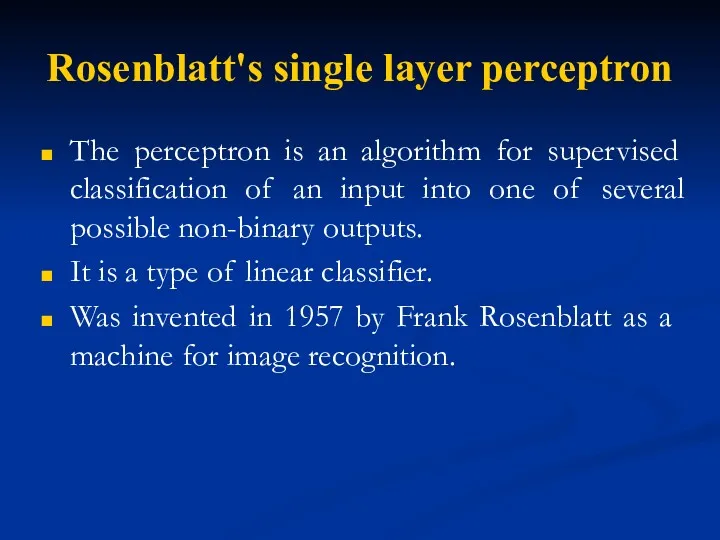
- 43. Rosenblatt's single layer perceptron The perceptron is an algorithm for supervised classification of an input into
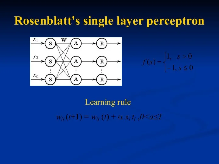
- 44. Rosenblatt's single layer perceptron Learning rule
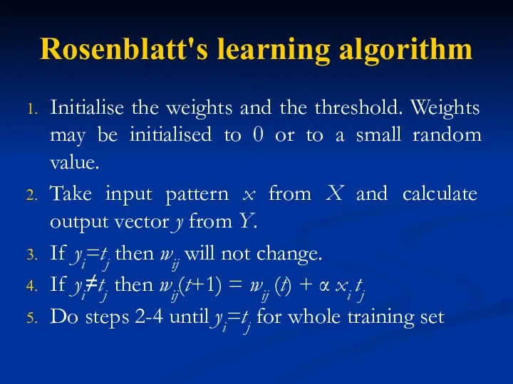
- 45. Rosenblatt's learning algorithm Initialise the weights and the threshold. Weights may be initialised to 0 or
- 46. Rosenblatt's single layer perceptron It was quickly proved that perceptrons could not be trained to recognize
- 47. Practice with Rosenblatt's perceptron Construction the linear classifier (Rosenblatt’s neural network perceptron) based on given training
- 48. Associative memory Associative memory (computer science) - a data-storage device in which a location is identified
- 49. Associative memory Autoassociative memories are capable of retrieving a piece of data upon presentation of only
- 50. Autoassociative memory based on sign activation function Neural network structure: Number of neurons in the input
- 51. Practice with autoassociative memory Realization of the associative memory based on sign activation function. Working with
- 52. Using single layer neural networks for time series forecasting A time series - sequence of data
- 53. Using single layer neural networks for time series forecasting Training samples
- 54. Practice with time series forecasting Using ADALINE neural networks for currency forecasting: Creation the training set
- 55. Multilayer perceptron
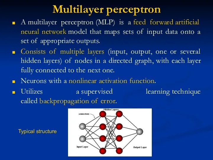
- 56. Multilayer perceptron A multilayer perceptron (MLP) is a feed forward artificial neural network model that maps
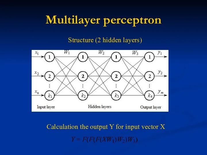
- 57. Multilayer perceptron Structure (2 hidden layers) Calculation the output Y for input vector X
- 58. Multilayer perceptron Activation function is not a threshold Usually a sigmoid function Function approximator Not limited
- 59. Classification ability A single layer network can only find a linear discriminant function. It can divide
- 60. Classification ability Universal Function Approximation Theorem MLP with one hidden layer can approximate arbitrarily closely every
- 61. Classification ability Any function can be approximated to arbitrary accuracy by a network with two hidden
- 62. Backpropagation algorithm D. Rumelhart, G. Hinton, R. Williams (1986) Most common method of obtaining the weights
- 63. Basic steps Forward propagation of a training pattern's input through the neural network in order to
- 64. Backpropagation
- 65. Backpropagation We use gradient descent method for minimizing the error
- 66. Backpropagation Theorem. For any hidden layer i of the neural network, error of the neuron i
- 67. Backpropagation Theorem. We can calculate derivatives of error E through the weights w and bias T
- 68. Backpropagation Backpropagation rule
- 69. Backpropagation algorithm Define the training speed α (0 Initialize the weights and biases by random way.
- 70. Backpropagation algorithm 4. Calculate overall error for all patterns 5. If E>Em then go to the
- 71. Practice. Calculation delta-rule expressions for various activation functions
- 72. Some problems The learning rate is important Too small Convergence extremely slow Too large May not
- 73. Some problems Overfitting The number of hidden neurons is very important, it defines the complexity of
- 74. What constitutes a “good” training set? Samples must represent the general population Samples must contain members
- 75. Practice with multilayer perceptron Using MLP for noisy digits recognition & Using MLP for time series
- 76. Recurrent neural networks Capable to influence to themselves by means of recurrences, e.g. by including the
- 77. Hopfield network 1. Invented by John Hopfield in 1982. 2. Content-addressable memory with binary threshold nodes
- 78. Hopfield network
- 79. Hopfield network as associative memory
- 80. Using hopfield network as associative memory
- 81. Hopfield network as associative memory Take noisy pattern y Realize iterations Until we will not reach
- 82. Example
- 83. Practice with Hopfield network Realization of the associative memory based on Hopfield Neural Network Working with
- 84. Hamming network R. Lippman (1987) Hamming network is two-network bipolar classifier. The first layer is single-layer
- 85. Hamming network
- 86. Hamming network working algorithm Define weights wij, Tj Get input pattern and initialize Hopfield weights Make
- 87. Self-organizing maps
- 88. Self-organizing maps Unsupervised Training The training set only consists of input patterns. The neural network adjusts
- 89. Self-organizing maps (SOM) A self-organizing map (SOM) is a type of artificial neural networkA self-organizing map
- 90. Self-organizing maps We only ask which neuron is active at the moment. We are not interested
- 92. Scheme of training of self-organizing map
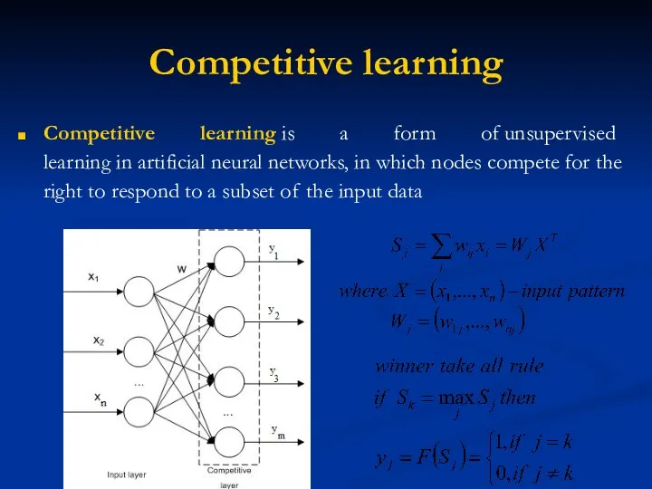
- 93. Competitive learning Competitive learning is a form of unsupervised learning in artificial neural networks, in which
- 94. Competitive learning
- 95. Vector quantization It works by dividing a large set of points (vectors) into groups having approximately
- 96. Vector quantization Choose random weights from [0;1]. t=1 Take all input patterns Xl,l=1,L t=t+1 Applications: data
- 97. Kohonen Maps
- 98. Kohonen maps
- 99. Kohonen maps learning procedure Choose random weights from [0;1]. t=1 Take input pattern Xl and calculate
- 100. Training and Testing
- 101. Training The goal is to achieve a balance between correct responses for the training patterns and
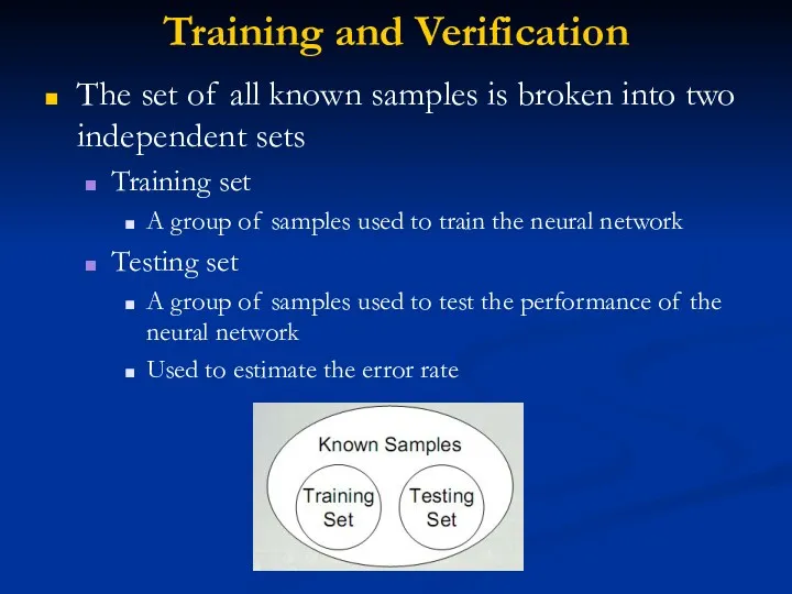
- 102. Training and Verification The set of all known samples is broken into two independent sets Training
- 103. Verification Provides an unbiased test of the quality of the network Common error is to “test”
- 104. Summary (Discussion) Artificial neural networks are inspired by the learning processes that take place in biological
- 105. Summary Learning tasks of artificial neural networks can be reformulated as function approximation tasks. Neural networks
- 106. Questions and Comments
- 108. Скачать презентацию
Table of contents
The basic concepts of neural networks
Artificial neural networks.
The
Table of contents
The basic concepts of neural networks
Artificial neural networks.
The
Self-organizing maps
The principle of unsupervised learning.
Kohonen self-organizing maps.
Learning Kohonen
Self-organizing maps
The principle of unsupervised learning.
Kohonen self-organizing maps.
Learning Kohonen
References
David Kriesel. A brief Introduction to Neural networks // http://www.dkriesel.com/en/science/neural_networks
Raul
References
David Kriesel. A brief Introduction to Neural networks // http://www.dkriesel.com/en/science/neural_networks
Raul
The basic concepts of neural networks
The basic concepts of neural networks
Questions for motivation discussion
What tasks are machines good at doing that
Questions for motivation discussion
What tasks are machines good at doing that
Types of learning
Knowledge acquisition from expert.
Knowledge acquisition from data:
Supervised learning –
Types of learning
Knowledge acquisition from expert.
Knowledge acquisition from data:
Supervised learning –
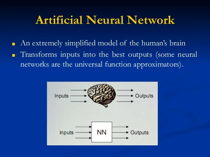
Artificial Neural Network
An extremely simplified model of the human’s brain
Transforms inputs
Artificial Neural Network
An extremely simplified model of the human’s brain
Transforms inputs
Artificial Neural Networks
Development of Neural Networks date back to the early
Artificial Neural Networks
Development of Neural Networks date back to the early
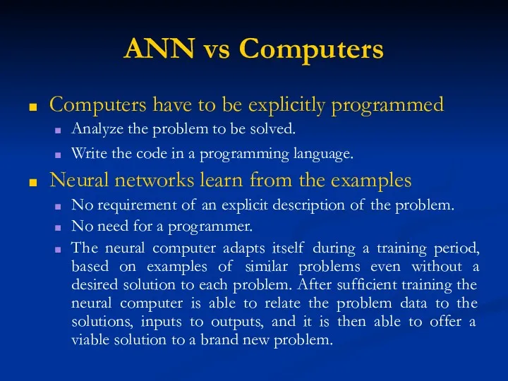
ANN vs Computers
Computers have to be explicitly programmed
Analyze the problem to
ANN vs Computers
Computers have to be explicitly programmed
Analyze the problem to
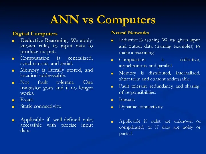
ANN vs Computers
Digital Computers
Deductive Reasoning. We apply known rules to input
ANN vs Computers
Digital Computers
Deductive Reasoning. We apply known rules to input
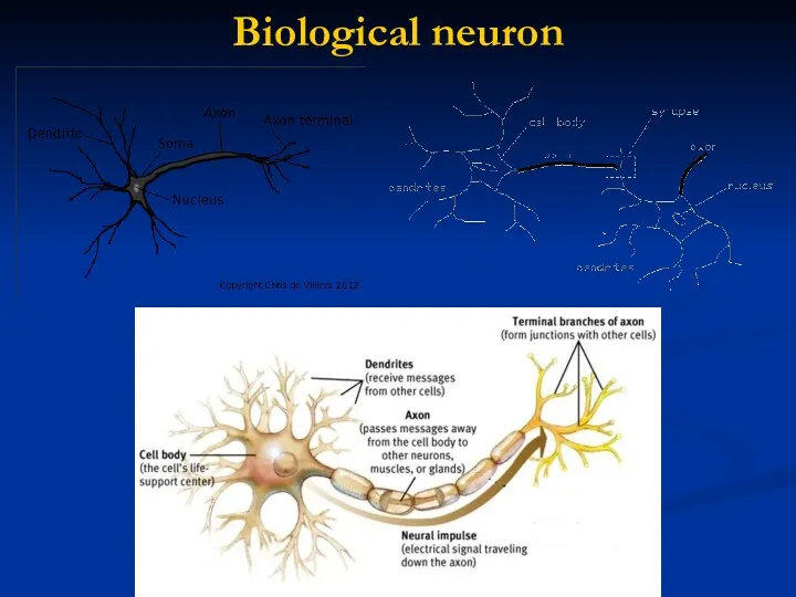
Biological neuron
Biological neuron
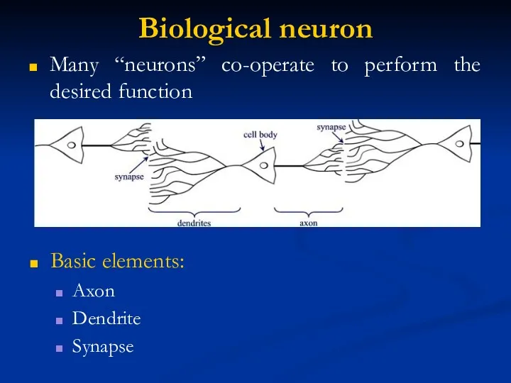
Biological neuron
Many “neurons” co-operate to perform the desired function
Basic elements:
Axon
Dendrite
Synapse
Biological neuron
Many “neurons” co-operate to perform the desired function
Basic elements:
Axon
Dendrite
Synapse
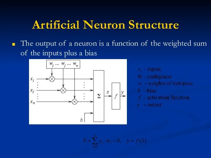
Artificial Neuron Structure
The output of a neuron is a function of
Artificial Neuron Structure
The output of a neuron is a function of
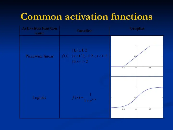
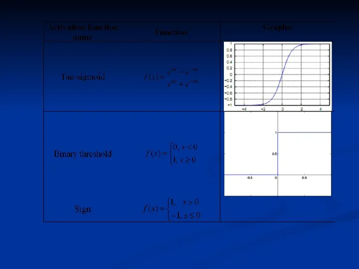
Common activation functions
Common activation functions
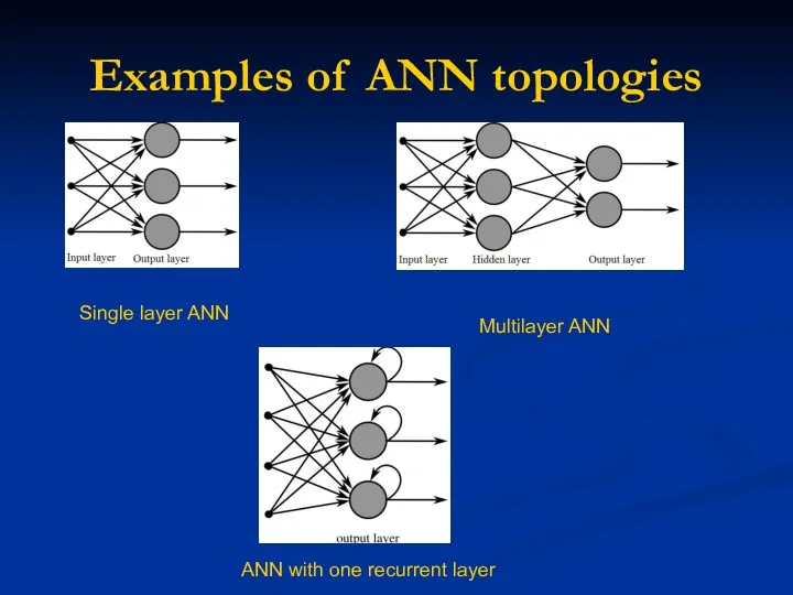
Examples of ANN topologies
Single layer ANN
Multilayer ANN
ANN with one recurrent layer
Examples of ANN topologies
Single layer ANN
Multilayer ANN
ANN with one recurrent layer
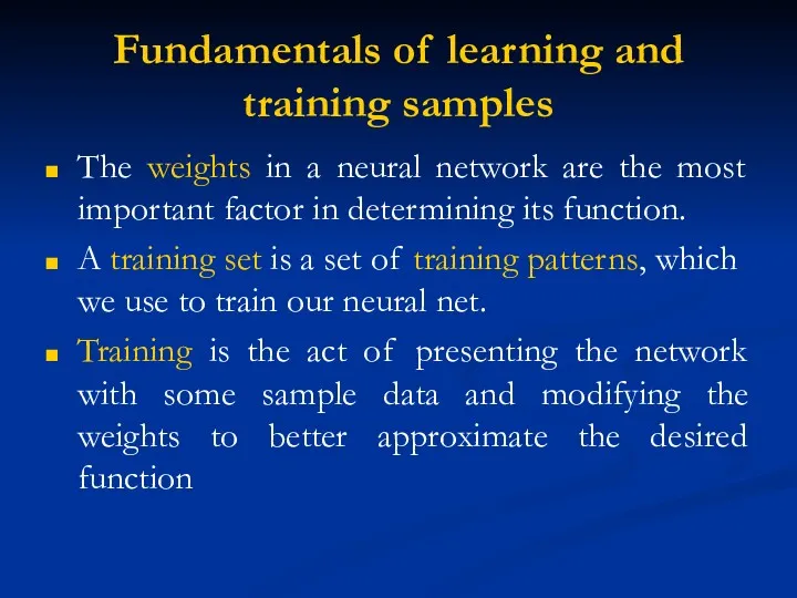
Fundamentals of learning and training samples
The weights in a neural
Fundamentals of learning and training samples
The weights in a neural
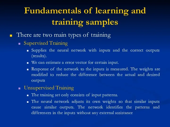
Fundamentals of learning and training samples
There are two main types
Fundamentals of learning and training samples
There are two main types
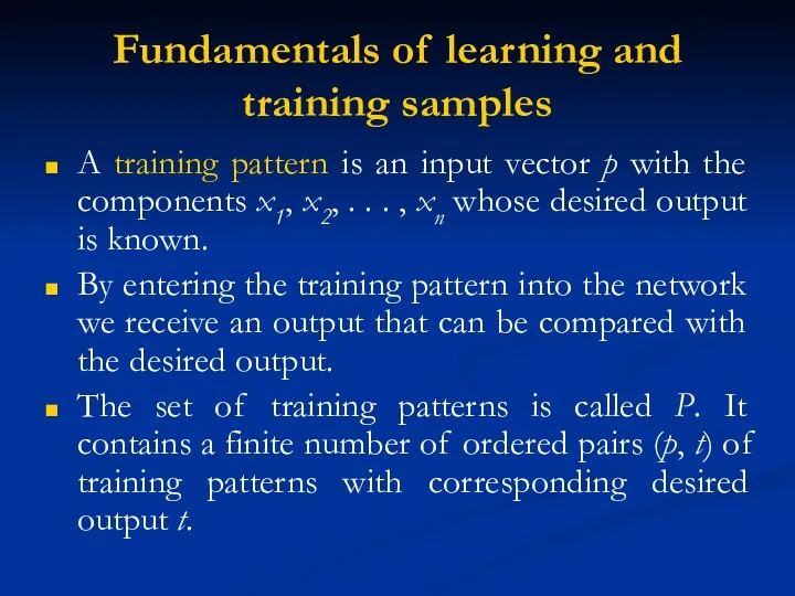
Fundamentals of learning and training samples
A training pattern is an
Fundamentals of learning and training samples
A training pattern is an
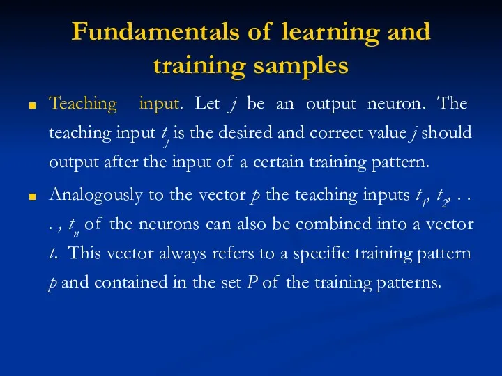
Fundamentals of learning and training samples
Teaching input. Let j be an
Fundamentals of learning and training samples
Teaching input. Let j be an
Fundamentals of learning and training samples
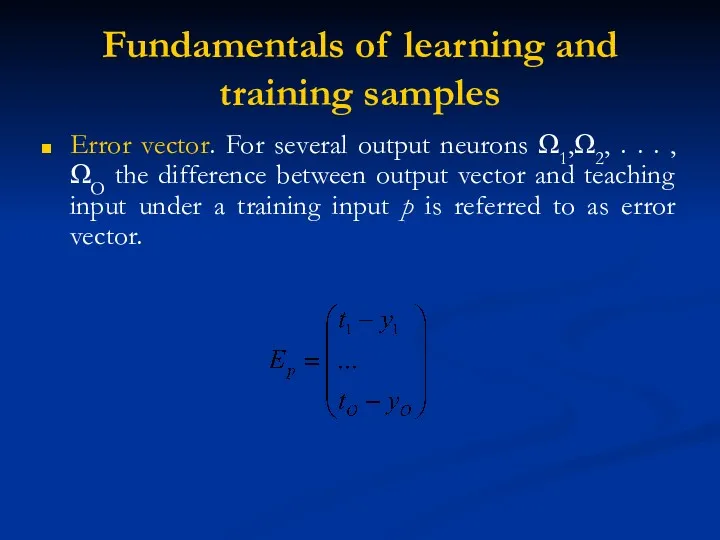
Error vector. For several output neurons
Fundamentals of learning and training samples
Error vector. For several output neurons
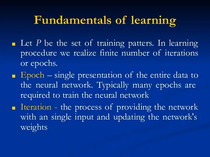
Fundamentals of learning
Let P be the set of training patters. In
Fundamentals of learning
Let P be the set of training patters. In
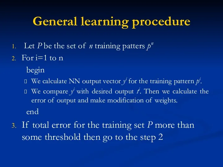
General learning procedure
Let P be the set of n training
General learning procedure
Let P be the set of n training
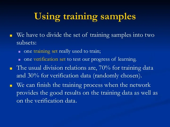
Using training samples
We have to divide the set of training samples
Using training samples
We have to divide the set of training samples
Learning curve
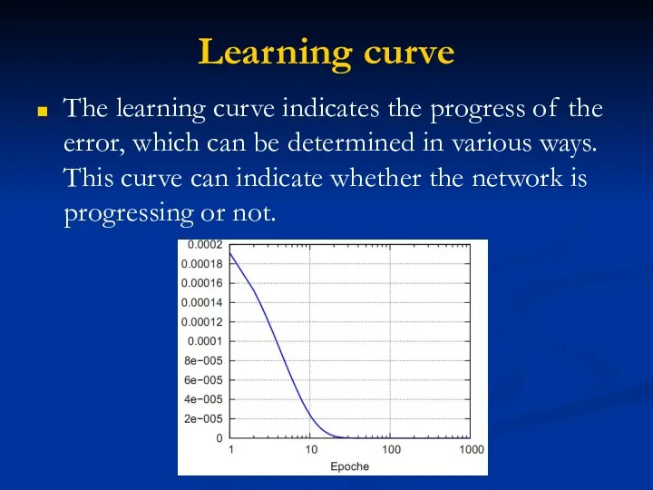
The learning curve indicates the progress of the error, which
Learning curve
The learning curve indicates the progress of the error, which
Error measurement
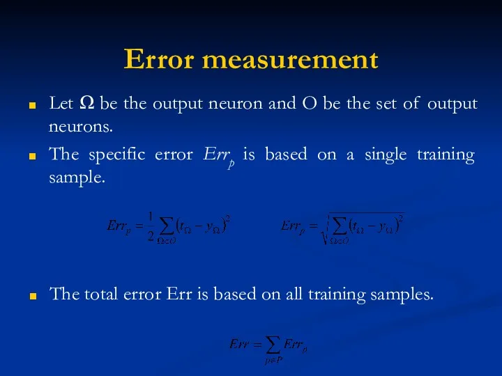
Let Ω be the output neuron and O be the
Error measurement
Let Ω be the output neuron and O be the
When do we stop learning?
Generally, the training process is stopped when
When do we stop learning?
Generally, the training process is stopped when
Using neural networks in practice (discussion)
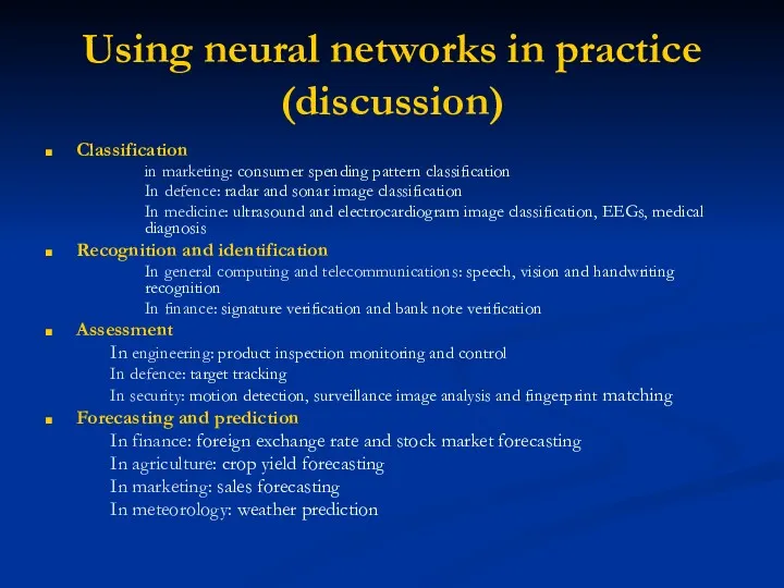
Classification
in marketing: consumer spending pattern
Using neural networks in practice (discussion)
Classification
in marketing: consumer spending pattern
Single layer neural networks
Single layer neural networks
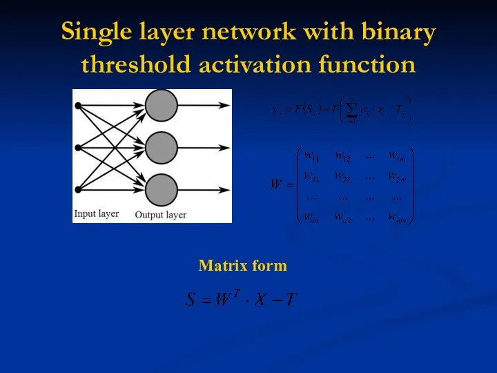
Single layer network with binary threshold activation function
Matrix form
Single layer network with binary threshold activation function
Matrix form
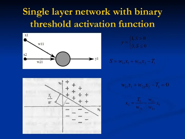
Single layer network with binary threshold activation function
Single layer network with binary threshold activation function
Practice with single layer
neural network
Performing a calculations in single
Practice with single layer
neural network
Performing a calculations in single
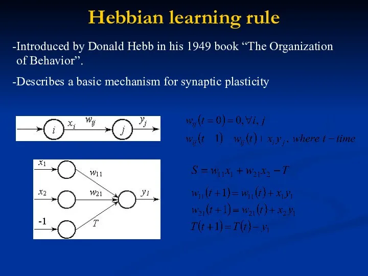
Hebbian learning rule
Introduced by Donald Hebb in his 1949 book “The Organization of Behavior”.
Hebbian learning rule
Introduced by Donald Hebb in his 1949 book “The Organization of Behavior”.
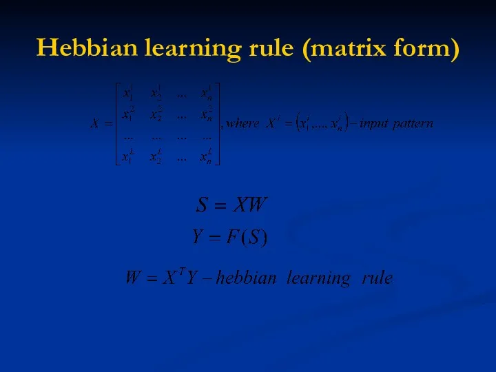
Hebbian learning rule (matrix form)
Hebbian learning rule (matrix form)
Practice with
hebbian learning rule
Construction the neural network based on hebbian
Practice with
hebbian learning rule
Construction the neural network based on hebbian
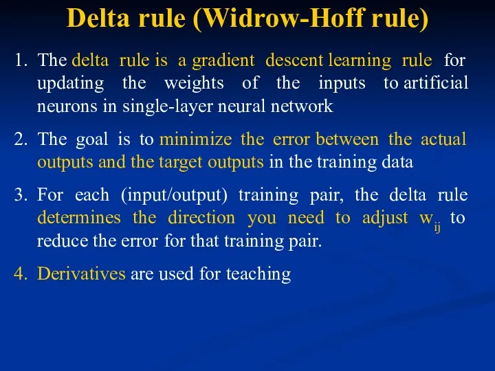
Delta rule (Widrow-Hoff rule)
The delta rule is a gradient descent learning rule for updating the
Delta rule (Widrow-Hoff rule)
The delta rule is a gradient descent learning rule for updating the
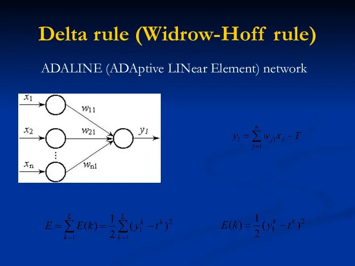
Delta rule (Widrow-Hoff rule)
ADALINE (ADAptive LINear Element) network
Delta rule (Widrow-Hoff rule)
ADALINE (ADAptive LINear Element) network
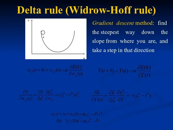
Delta rule (Widrow-Hoff rule)
Gradient descent method: find the steepest way down the slope from
Delta rule (Widrow-Hoff rule)
Gradient descent method: find the steepest way down the slope from
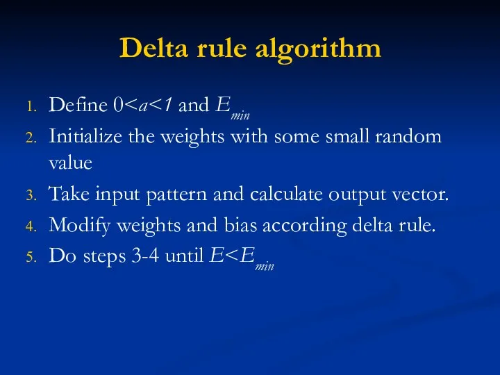
Delta rule algorithm
Define 0Initialize the weights with some
Delta rule algorithm
Define 0
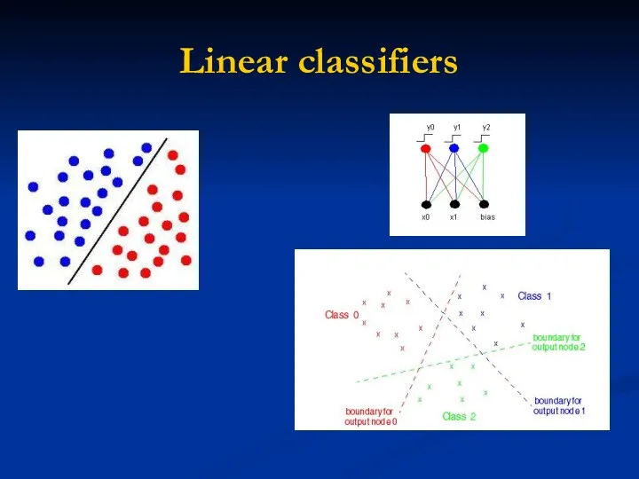
Linear classifiers
Linear classifiers
Practice with delta rule
Construction the ADALINE neural network (linear classifier
Practice with delta rule
Construction the ADALINE neural network (linear classifier
Rosenblatt's single layer perceptron
The perceptron is an algorithm for supervised classification
Rosenblatt's single layer perceptron
The perceptron is an algorithm for supervised classification
Rosenblatt's single layer perceptron
Learning rule
Rosenblatt's single layer perceptron
Learning rule
Rosenblatt's learning algorithm
Initialise the weights and the threshold. Weights may be
Rosenblatt's learning algorithm
Initialise the weights and the threshold. Weights may be
Rosenblatt's single layer perceptron
It was quickly proved that perceptrons could not
Rosenblatt's single layer perceptron
It was quickly proved that perceptrons could not
Practice with Rosenblatt's perceptron
Construction the linear classifier (Rosenblatt’s neural network perceptron)
Practice with Rosenblatt's perceptron
Construction the linear classifier (Rosenblatt’s neural network perceptron)
Associative memory
Associative memory (computer science) - a data-storage device in which
Associative memory
Associative memory (computer science) - a data-storage device in which
Associative memory
Autoassociative memories are capable of retrieving a piece of data
Associative memory
Autoassociative memories are capable of retrieving a piece of data
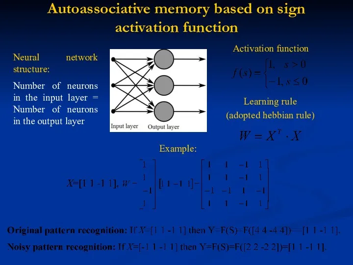
Autoassociative memory based on sign activation function
Neural network structure:
Number of neurons
Autoassociative memory based on sign activation function
Neural network structure:
Number of neurons
Practice with autoassociative memory
Realization of the associative memory based on sign
Practice with autoassociative memory
Realization of the associative memory based on sign
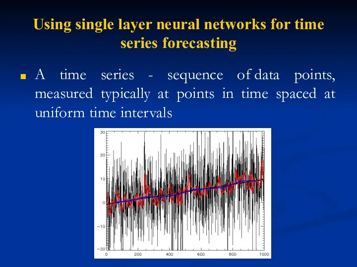
Using single layer neural networks for time series forecasting
A time series
Using single layer neural networks for time series forecasting
A time series
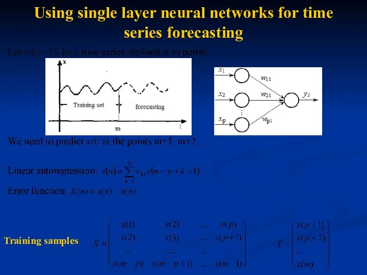
Using single layer neural networks for time series forecasting
Training samples
Using single layer neural networks for time series forecasting
Training samples
Practice with
time series forecasting
Using ADALINE neural networks for currency forecasting:
Creation
Practice with
time series forecasting
Using ADALINE neural networks for currency forecasting:
Creation
Multilayer perceptron
Multilayer perceptron
Multilayer perceptron
A multilayer perceptron (MLP) is a feed forward artificial neural network model that maps sets
Multilayer perceptron
A multilayer perceptron (MLP) is a feed forward artificial neural network model that maps sets
Multilayer perceptron
Structure (2 hidden layers)
Calculation the output Y for input vector
Multilayer perceptron
Structure (2 hidden layers)
Calculation the output Y for input vector
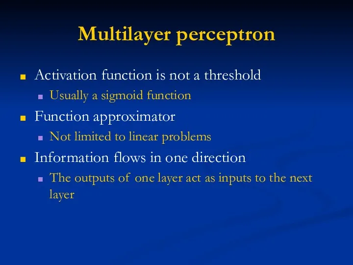
Multilayer perceptron
Activation function is not a threshold
Usually a sigmoid function
Function approximator
Not
Multilayer perceptron
Activation function is not a threshold
Usually a sigmoid function
Function approximator
Not
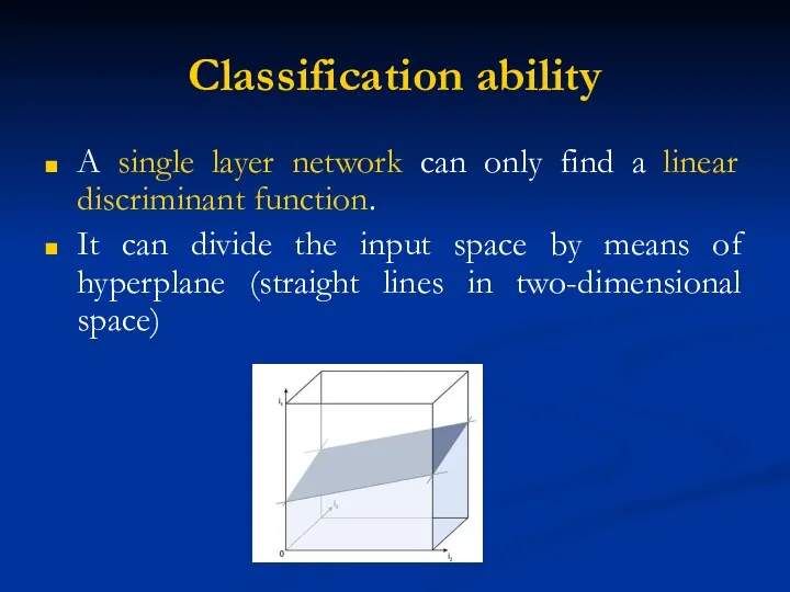
Classification ability
A single layer network can only find a linear discriminant
Classification ability
A single layer network can only find a linear discriminant
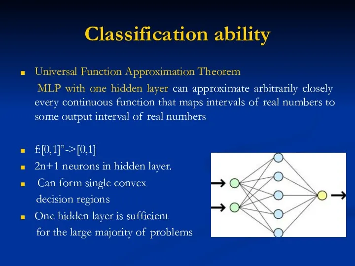
Classification ability
Universal Function Approximation Theorem
MLP with one hidden layer
Classification ability
Universal Function Approximation Theorem
MLP with one hidden layer
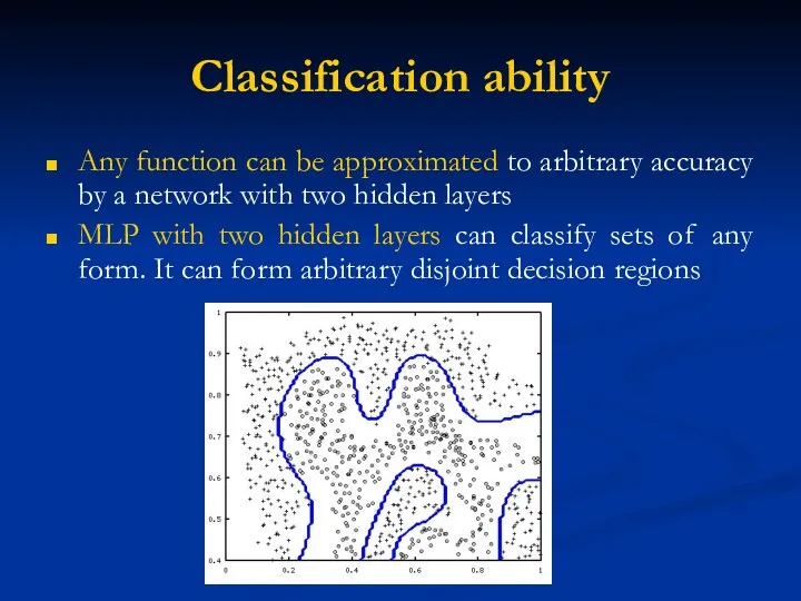
Classification ability
Any function can be approximated to arbitrary accuracy by a
Classification ability
Any function can be approximated to arbitrary accuracy by a
Backpropagation algorithm
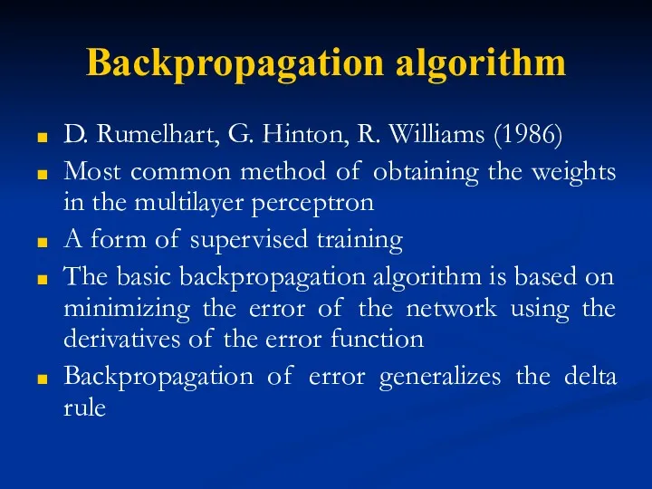
D. Rumelhart, G. Hinton, R. Williams (1986)
Most common method of
Backpropagation algorithm
D. Rumelhart, G. Hinton, R. Williams (1986)
Most common method of
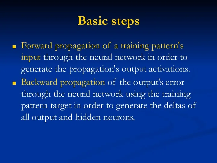
Basic steps
Forward propagation of a training pattern's input through the neural
Basic steps
Forward propagation of a training pattern's input through the neural
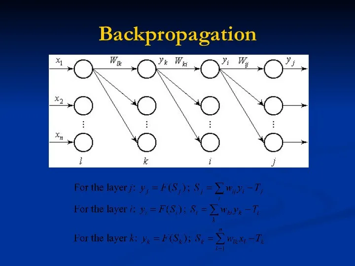
Backpropagation
Backpropagation
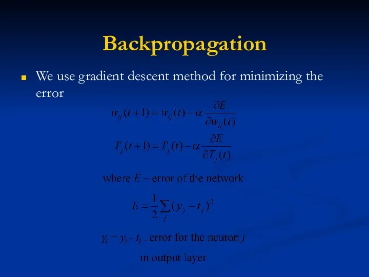
Backpropagation
We use gradient descent method for minimizing the error
Backpropagation
We use gradient descent method for minimizing the error
Backpropagation
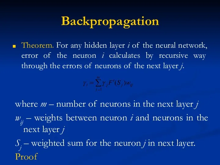
Theorem. For any hidden layer i of the neural network, error
Backpropagation
Theorem. For any hidden layer i of the neural network, error
Backpropagation
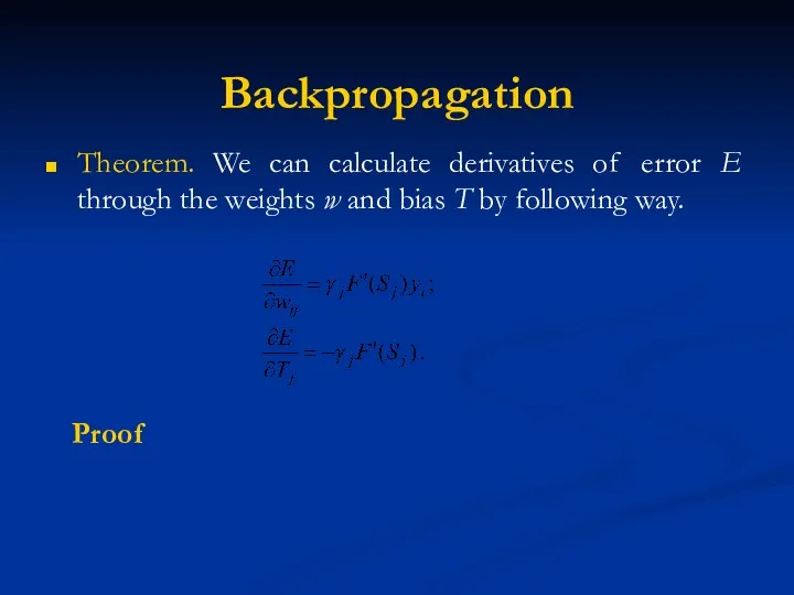
Theorem. We can calculate derivatives of error E through the weights
Backpropagation
Theorem. We can calculate derivatives of error E through the weights
Backpropagation
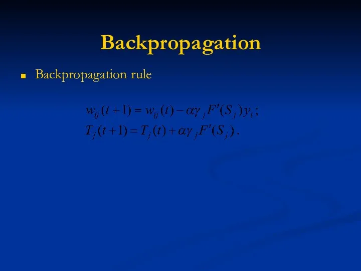
Backpropagation rule
Backpropagation
Backpropagation rule
Backpropagation algorithm
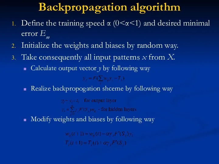
Define the training speed α (0<α<1) and desired minimal error
Backpropagation algorithm
Define the training speed α (0<α<1) and desired minimal error
Backpropagation algorithm
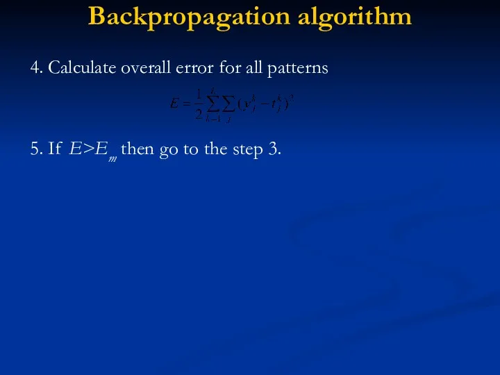
4. Calculate overall error for all patterns
5. If E>Em then
Backpropagation algorithm
4. Calculate overall error for all patterns
5. If E>Em then
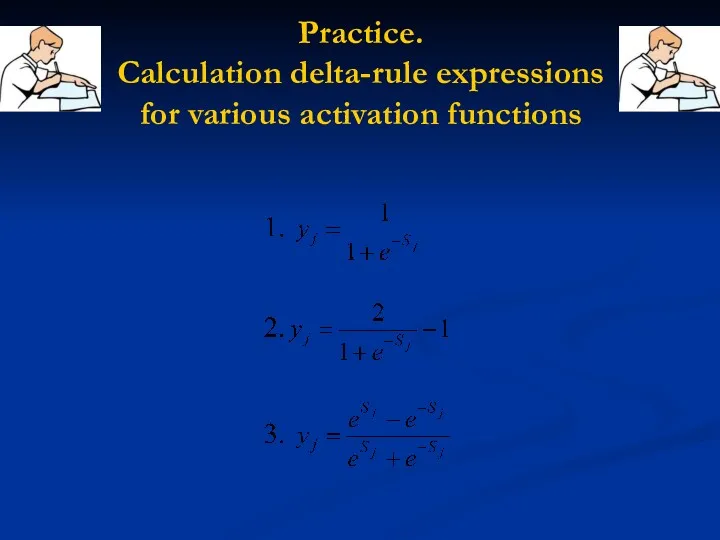
Practice.
Calculation delta-rule expressions
for various activation functions
Practice.
Calculation delta-rule expressions
for various activation functions
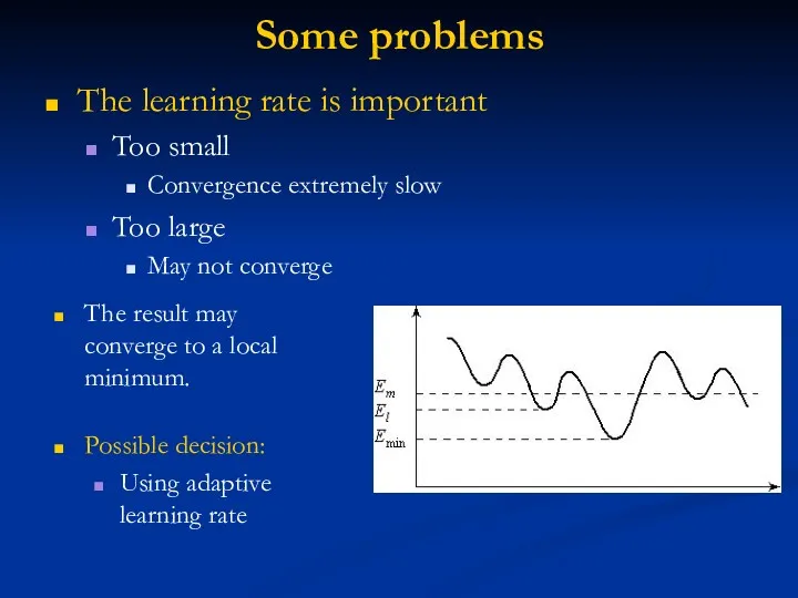
Some problems
The learning rate is important
Too small
Convergence extremely slow
Too large
May not
Some problems
The learning rate is important
Too small
Convergence extremely slow
Too large
May not
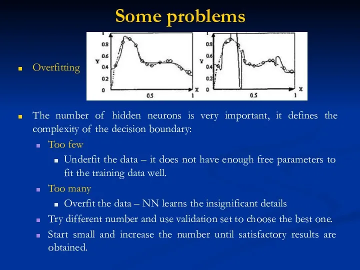
Some problems
Overfitting
The number of hidden neurons is very important, it defines
Some problems
Overfitting
The number of hidden neurons is very important, it defines
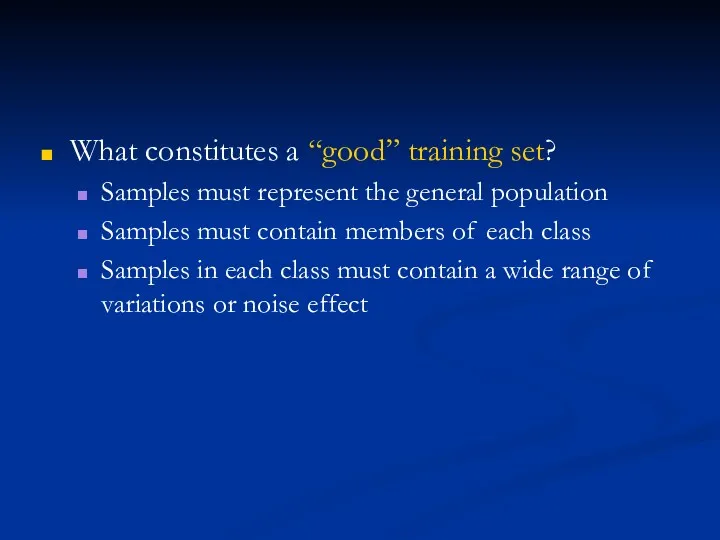
What constitutes a “good” training set?
Samples must represent the general population
Samples
What constitutes a “good” training set?
Samples must represent the general population
Samples
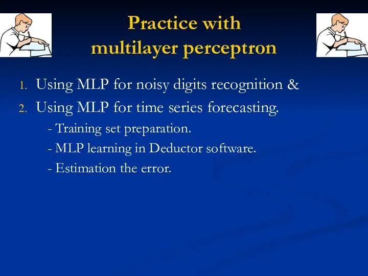
Practice with
multilayer perceptron
Using MLP for noisy digits recognition &
Using MLP
Practice with
multilayer perceptron
Using MLP for noisy digits recognition &
Using MLP
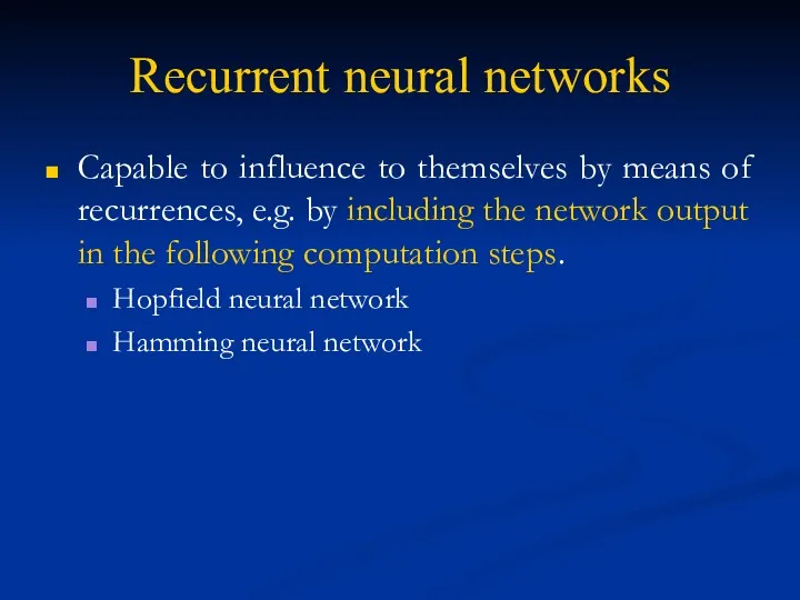
Recurrent neural networks
Capable to influence to themselves by means of recurrences,
Recurrent neural networks
Capable to influence to themselves by means of recurrences,
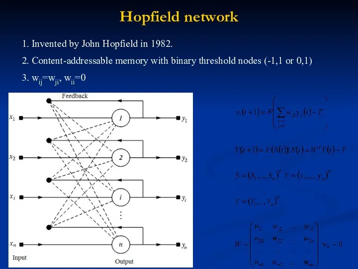
Hopfield network
1. Invented by John Hopfield in 1982.
2. Content-addressable memory with binary threshold nodes (-1,1 or
Hopfield network
1. Invented by John Hopfield in 1982.
2. Content-addressable memory with binary threshold nodes (-1,1 or
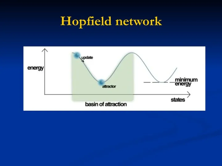
Hopfield network
Hopfield network
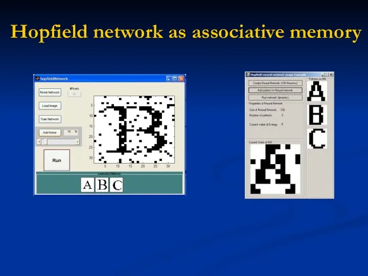
Hopfield network as associative memory
Hopfield network as associative memory
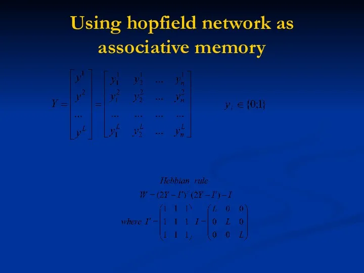
Using hopfield network as associative memory
Using hopfield network as associative memory
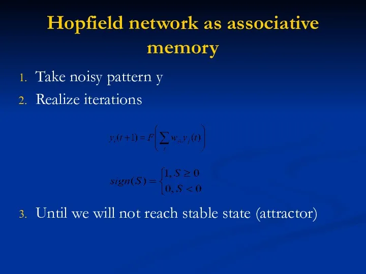
Hopfield network as associative memory
Take noisy pattern y
Realize iterations
Until we will
Hopfield network as associative memory
Take noisy pattern y
Realize iterations
Until we will
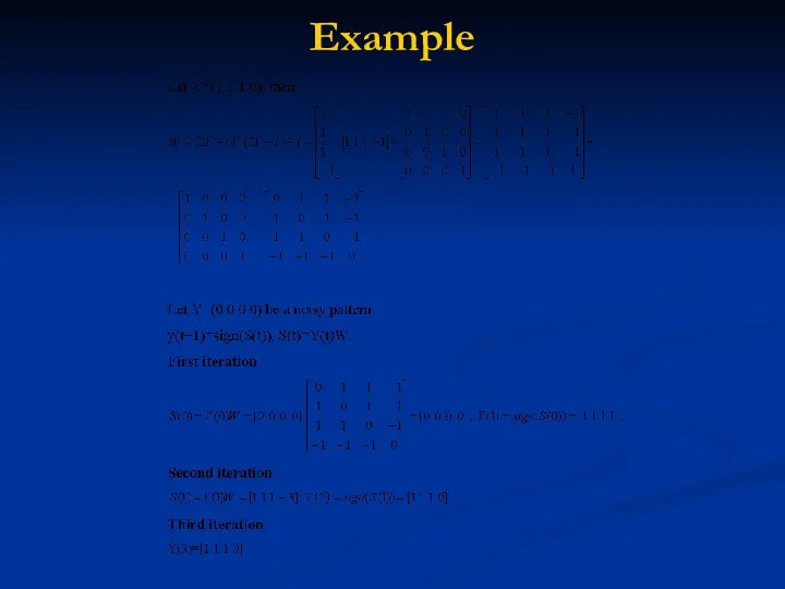
Example
Example
Practice
with Hopfield network
Realization of the associative memory based on Hopfield
Practice
with Hopfield network
Realization of the associative memory based on Hopfield
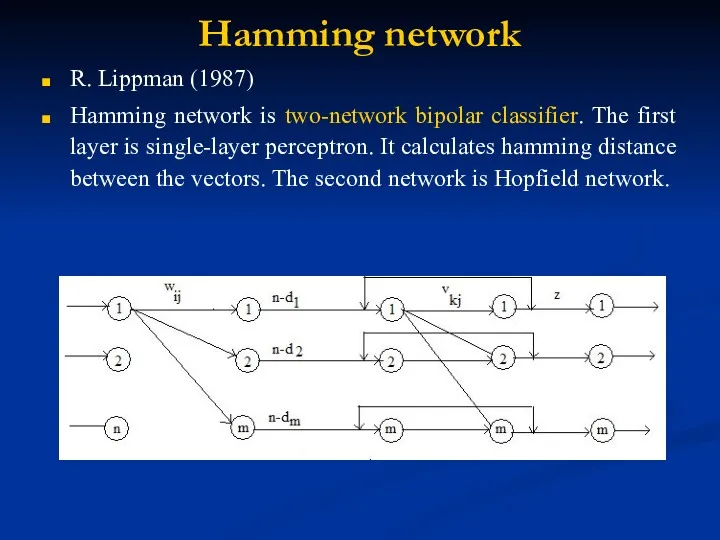
Hamming network
R. Lippman (1987)
Hamming network is two-network bipolar classifier. The first
Hamming network
R. Lippman (1987)
Hamming network is two-network bipolar classifier. The first
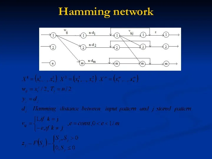
Hamming network
Hamming network
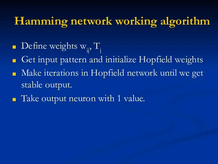
Hamming network working algorithm
Define weights wij, Tj
Get input pattern and initialize
Hamming network working algorithm
Define weights wij, Tj
Get input pattern and initialize

Self-organizing maps
Self-organizing maps
Self-organizing maps
Unsupervised Training
The training set only consists of input patterns.
The neural
Self-organizing maps
Unsupervised Training
The training set only consists of input patterns.
The neural
Self-organizing maps (SOM)
A self-organizing map (SOM) is a type of artificial neural networkA self-organizing map (SOM)
Self-organizing maps (SOM)
A self-organizing map (SOM) is a type of artificial neural networkA self-organizing map (SOM)
Self-organizing maps
We only ask which neuron is active at the moment.
We
Self-organizing maps
We only ask which neuron is active at the moment.
We

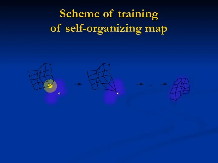
Scheme of training
of self-organizing map
Scheme of training
of self-organizing map
Competitive learning
Competitive learning is a form of unsupervised learning in artificial neural networks, in which
Competitive learning
Competitive learning is a form of unsupervised learning in artificial neural networks, in which
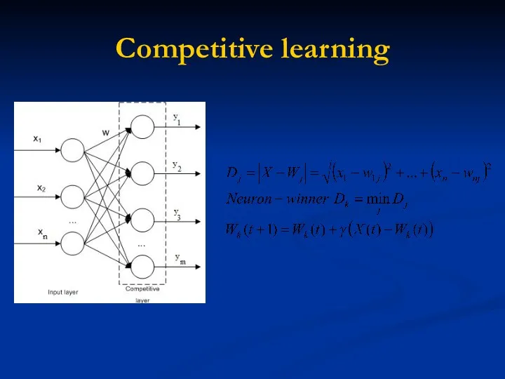
Competitive learning
Competitive learning
Vector quantization
It works by dividing a large set of points (vectors)
Vector quantization
It works by dividing a large set of points (vectors)
![Vector quantization Choose random weights from [0;1]. t=1 Take all](/_ipx/f_webp&q_80&fit_contain&s_1440x1080/imagesDir/jpg/5086/slide-95.jpg)
Vector quantization
Choose random weights from [0;1].
t=1
Take all input patterns Xl,l=1,L
t=t+1
Applications:
data compression
Vector quantization
Choose random weights from [0;1].
t=1
Take all input patterns Xl,l=1,L
t=t+1
Applications:
data compression
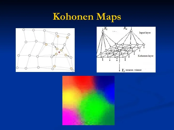
Kohonen Maps
Kohonen Maps
Kohonen maps
Kohonen maps
![Kohonen maps learning procedure Choose random weights from [0;1]. t=1](/_ipx/f_webp&q_80&fit_contain&s_1440x1080/imagesDir/jpg/5086/slide-98.jpg)
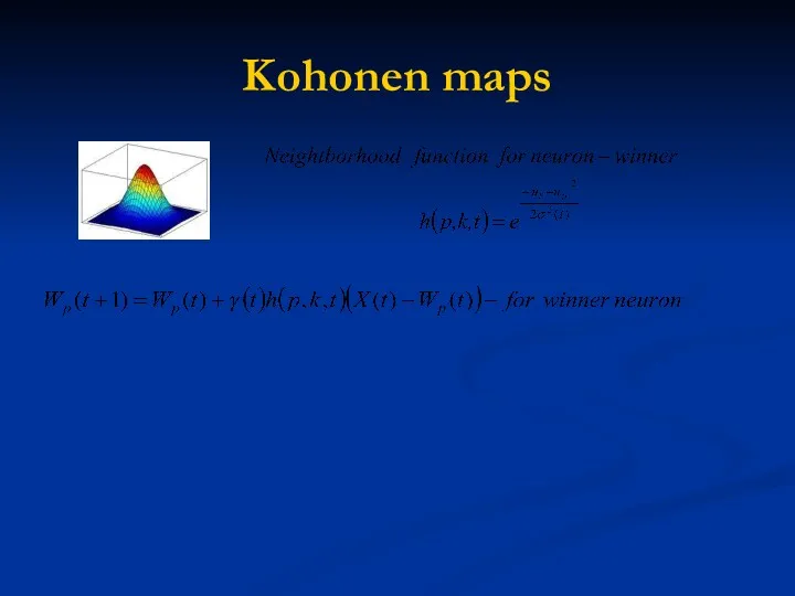
Kohonen maps learning procedure
Choose random weights from [0;1].
t=1
Take input pattern Xl
Kohonen maps learning procedure
Choose random weights from [0;1].
t=1
Take input pattern Xl
Training and Testing
Training and Testing
Training
The goal is to achieve a balance between correct responses for
Training
The goal is to achieve a balance between correct responses for
Training and Verification
The set of all known samples is broken into
Training and Verification
The set of all known samples is broken into

Verification
Provides an unbiased test of the quality of the network
Common
Verification
Provides an unbiased test of the quality of the network
Common
Summary (Discussion)
Artificial neural networks are inspired by the learning processes that
Summary (Discussion)
Artificial neural networks are inspired by the learning processes that
Summary
Learning tasks of artificial neural networks can be reformulated as function
Summary
Learning tasks of artificial neural networks can be reformulated as function

Questions and Comments
Questions and Comments
 SQL тілі: мәліметтермен жұмыс. Сұраныс құру
 Общее представление о информационных системах
 Кодирование звуковой информации
 Интернет-заработок для студентов
 Медиа-карта региона: федеральные СМИ
 Сто к одному. Игра
 Графические редакторы
 Базы данных. Основы проектирования баз данных. (Лекция 1)
 Алгоритм и его свойства. Примеры алгоритмов
 Обработка информации. Получение новой информации. 5 класс.
 Использование информационно-коммуникационных технологий в процессе обучения физике
 Основы программирования. Введение
 Информационные ресурсы и сервисы интернета
 Электронная цифровая подпись
 Kuplinov Play (популярный летсплейщик)
 Архитектура современного компьютера
 Компьютердің конструктивті құрылғылары
 Символьные данные и строки. Лекция 15а-15б
 Наследование. Основы наследования. Лекция №8
 Роботтехникасы. Гуманоид роботтар
 Протоколы обмена для линий последовательной передачи данных
 Сетевые характеристики. Лекция 6
 Big Data без космоса Как настроить и масштабировать работу с данными, если вы не Google… и даже не Yandex
 Отладка и пуск. Siemens
 Разработка информационной системы для творческой студии ИП Favorite
 Петербургский дневник
 Программирование на языке Python
 Оптимальное планирование