Solving ultimate pit limit problem through graph closure (L-G algorithm) and the fundamental tree algorithm презентация
- Solving ultimate pit limit problem through graph closure (L-G algorithm) and the fundamental tree algorithm

Содержание
- 2. Contents 1. Introduction 2. Lerchs – Grossmann (Graph closure) 3. Fundamental Tree Algorithm 4. Assignment
- 3. Introduction Two ojectives for open pit optimization Design ultimate pit limits (Moving cone, LG, Net work
- 4. Block model gdg Source: William Hustrulid: Open Pit Mine Planning & Design
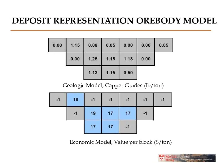
- 5. DEPOSIT REPRESENTATION OREBODY MODEL A set of mining blocks of a given size with block value
- 6. DEPOSIT REPRESENTATION OREBODY MODEL Geologic Model, Copper Grades (lb/ton) Economic Model, Value per block ($/ton)
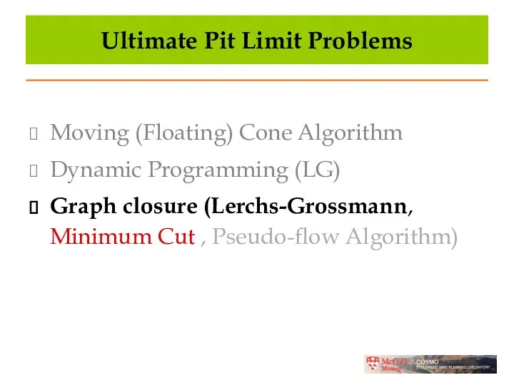
- 7. Ultimate Pit Limit Problems Moving (Floating) Cone Algorithm Dynamic Programming (LG) Graph closure (Lerchs-Grossmann, Minimum Cut
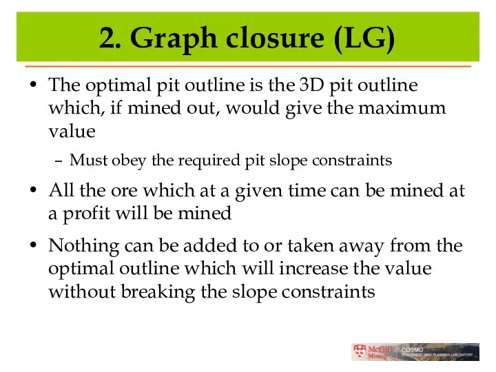
- 8. 2. Graph closure (LG) The optimal pit outline is the 3D pit outline which, if mined
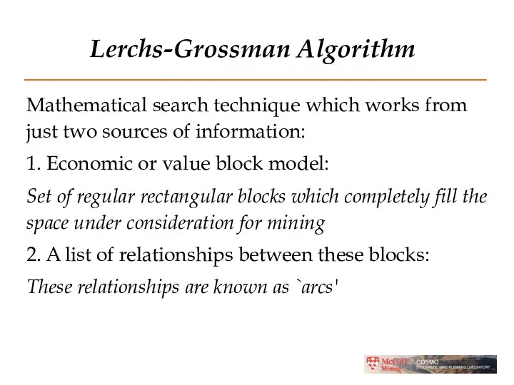
- 9. Lerchs-Grossman Algorithm Mathematical search technique which works from just two sources of information: 1. Economic or
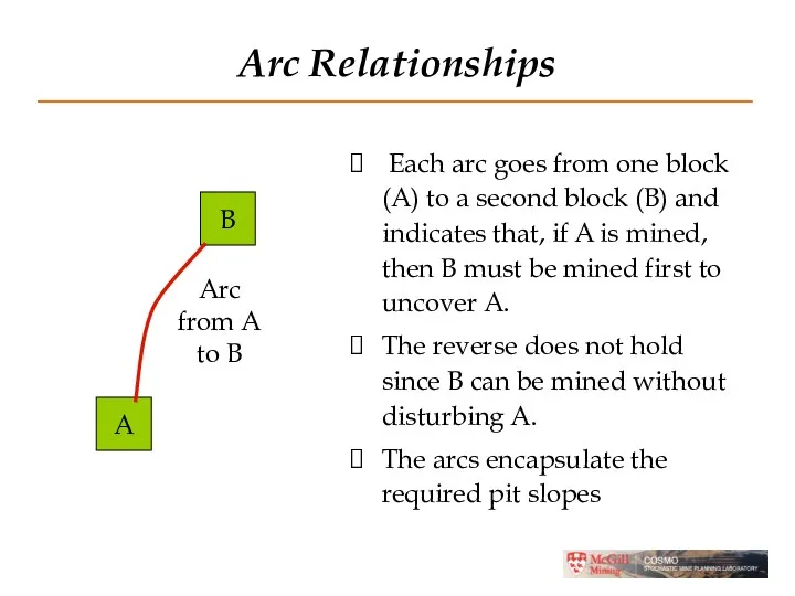
- 10. Arc Relationships Each arc goes from one block (A) to a second block (B) and indicates
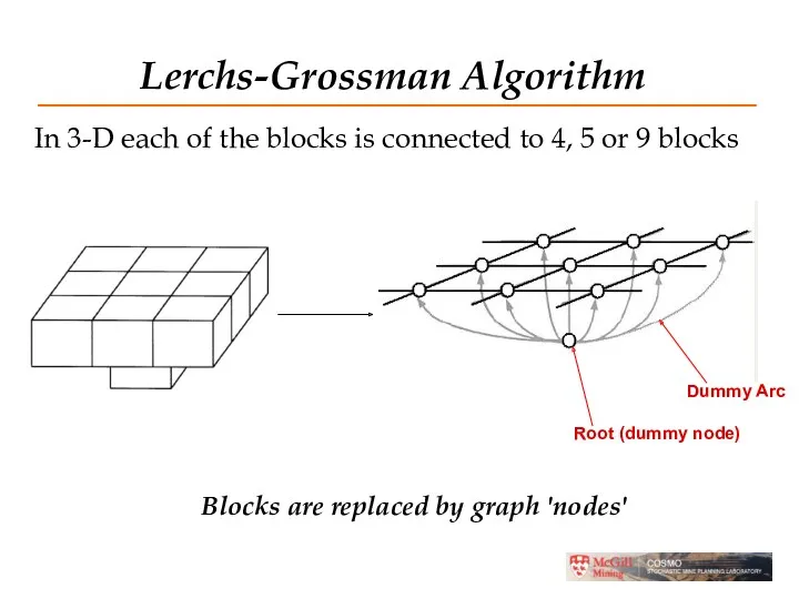
- 11. Lerchs-Grossman Algorithm In 3-D each of the blocks is connected to 4, 5 or 9 blocks
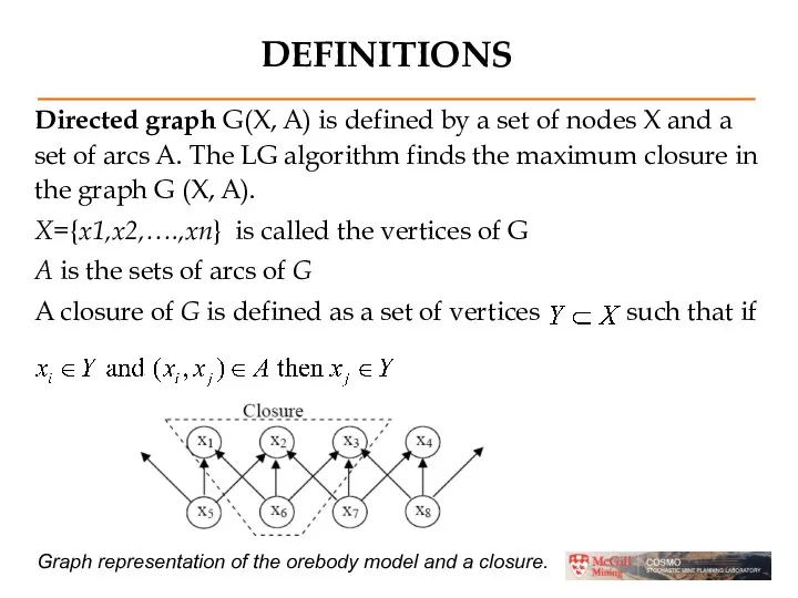
- 12. DEFINITIONS Directed graph G(X, A) is defined by a set of nodes X and a set
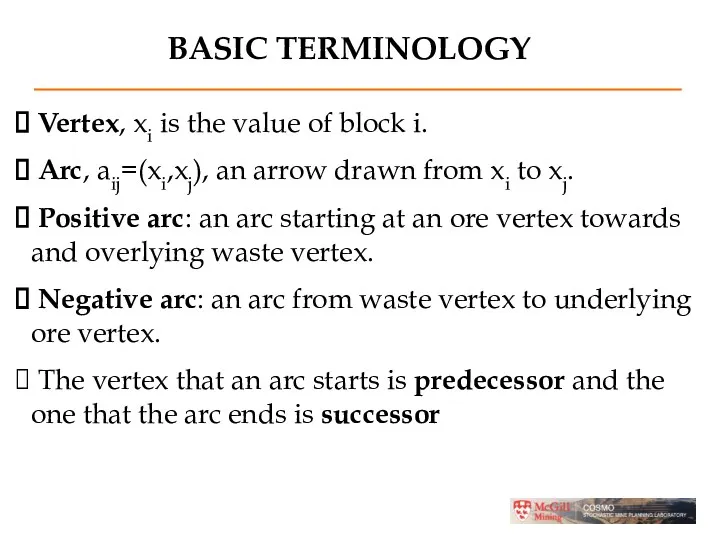
- 13. BASIC TERMINOLOGY Vertex, xi is the value of block i. Arc, aij=(xi,xj), an arrow drawn from
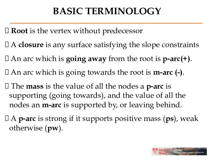
- 14. Root is the vertex without predecessor A closure is any surface satisfying the slope constraints An
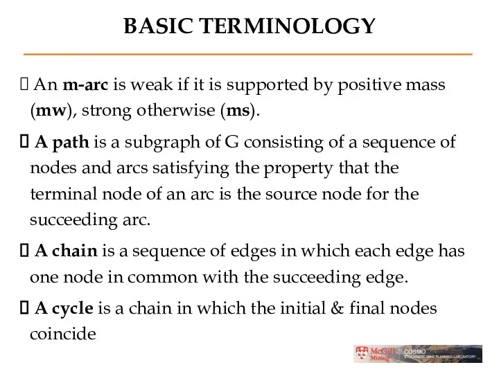
- 15. An m-arc is weak if it is supported by positive mass (mw), strong otherwise (ms). A
- 16. Example of LG -3 -4 +6 +9 X0 p-s m-w p-w p-s Root node
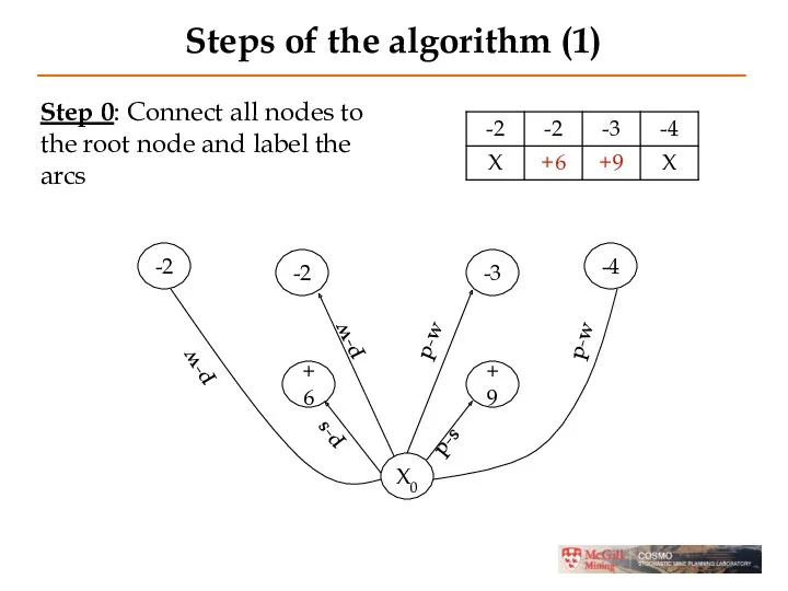
- 17. Steps of the algorithm (1) -2 -2 -3 -4 +6 +9 X0 Step 0: Connect all
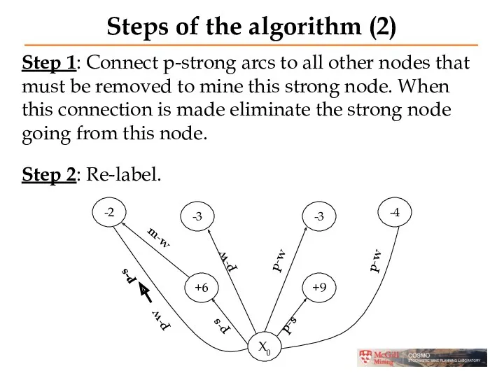
- 18. Steps of the algorithm (2) -2 -3 -3 -4 +6 +9 X0 Step 1: Connect p-strong
- 19. Step 3: Normalize the tree. Root (x0) must be common to all strong edges, if not,
- 20. Application of the steps for small orebody model Step 0:
- 21. Application of the steps … Step 1 and 2:
- 22. Application of the steps … Step 1-2 -1 -2 -1 -2 +4 +5 X0 p-w p-w
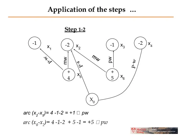
- 23. Application of the steps … Step 1-2 -1 -2 -1 -2 +4 +5 X0 mw p-w
- 24. Application of the steps … Step 1-2 arc (x0-x2)= 4 -1-2 + 5 -1-2= +3 ?
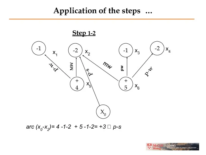
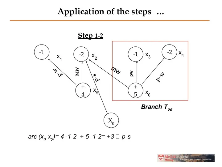
- 25. Application of the steps … Step 1-2 -1 -2 -1 -2 +4 +5 X0 mw p-w
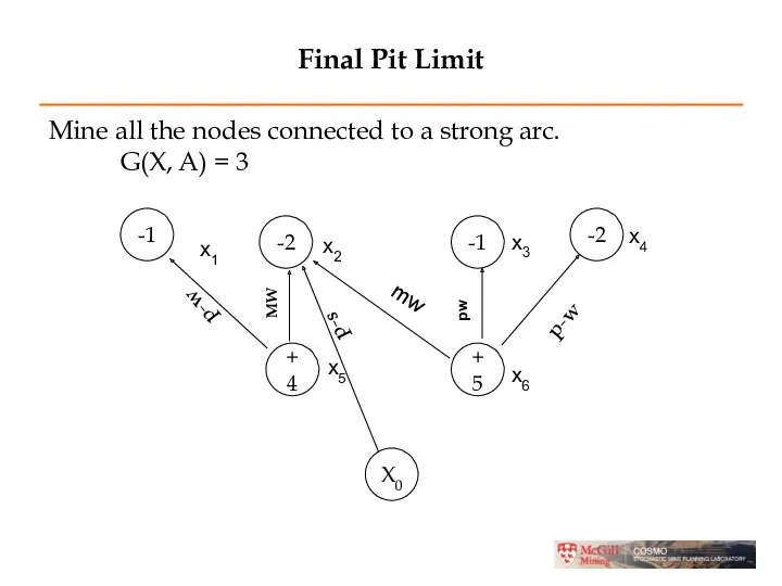
- 26. Final Pit Limit Mine all the nodes connected to a strong arc. G(X, A) = 3
- 27. Optimal Pit The L-G algorithm will flag each block as being inside or outside the optimal
- 28. Varying Slope Angles It is possible to have different slope angles in different areas of the
- 29. 3. Fundamental Tree Algorithm Long-term production scheduling consists of determining an optimal sequence of extracting the
- 30. The Approach To simplify the MIP we would like to decrease the number of blocks in
- 31. The Approach A Fundamental Tree is defined as a combination of blocks such that: The blocks
- 32. 3.1. Fundamental Tree Algorithm
- 33. Step 1 - Generate a Starting Network Given a our pushback block model represent blocks by
- 34. Example of Generating a Starting Network Example 2-D block model, shows the node numbers and the
- 35. Step 2 - Find the Cone Value The "cone" value of a block (CVi) is the
- 36. Step 3 – Assign cofficients to the Positive Nodes Each positive node will be assigned a
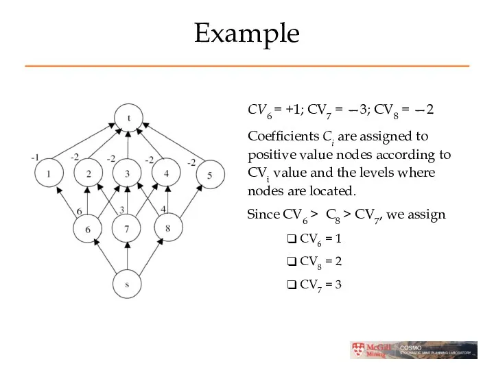
- 37. Example CV6 = +1; CV7 = —3; CV8 = —2 Coefficients Ci are assigned to positive
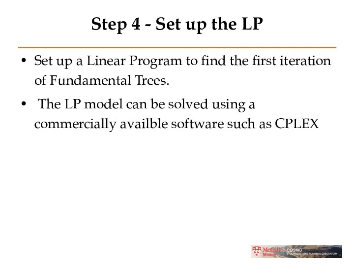
- 38. Step 4 - Set up the LP Set up a Linear Program to find the first
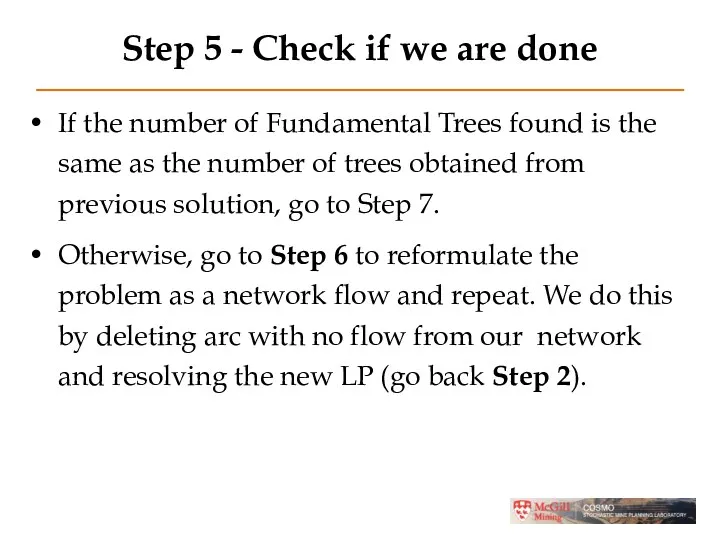
- 39. Step 5 - Check if we are done If the number of Fundamental Trees found is
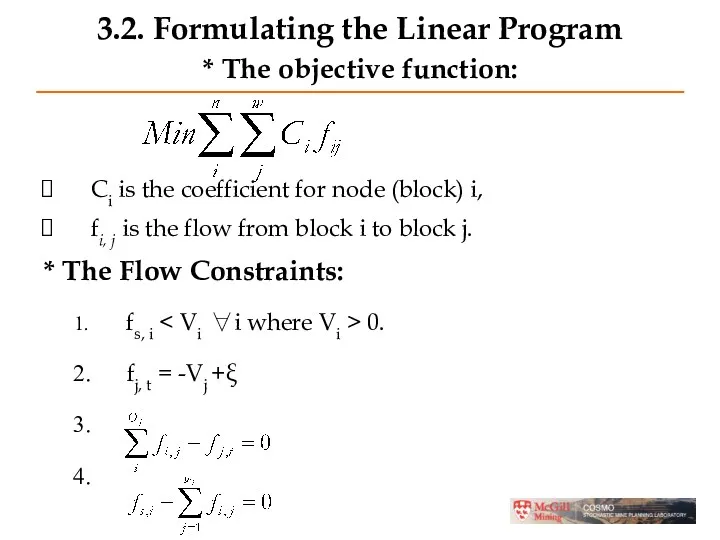
- 40. 3.2. Formulating the Linear Program * The objective function: Ci is the coefficient for node (block)
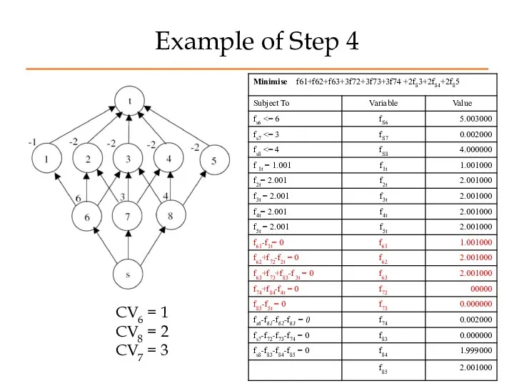
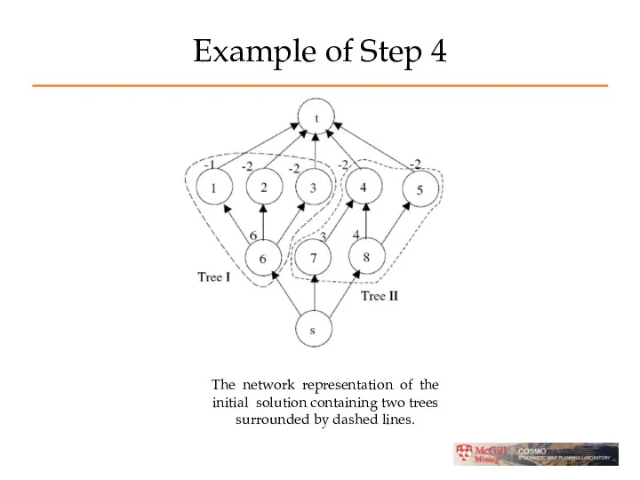
- 41. Example of Step 4
- 42. Example of Step 4 The network representation of the initial solution containing two trees surrounded by
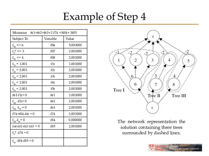
- 43. Example of Step 4 The network representation the solution containing three trees surrounded by dashed lines.
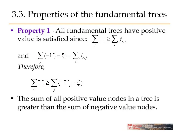
- 44. 3.3. Properties of the fundamental trees Property 1 - All fundamental trees have positive value is
- 45. Property 2 of the fundamental trees All fundamental trees obey the slope constraints if they are
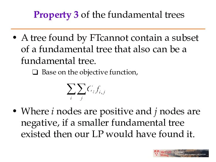
- 46. Property 3 of the fundamental trees A tree found by FTcannot contain a subset of a
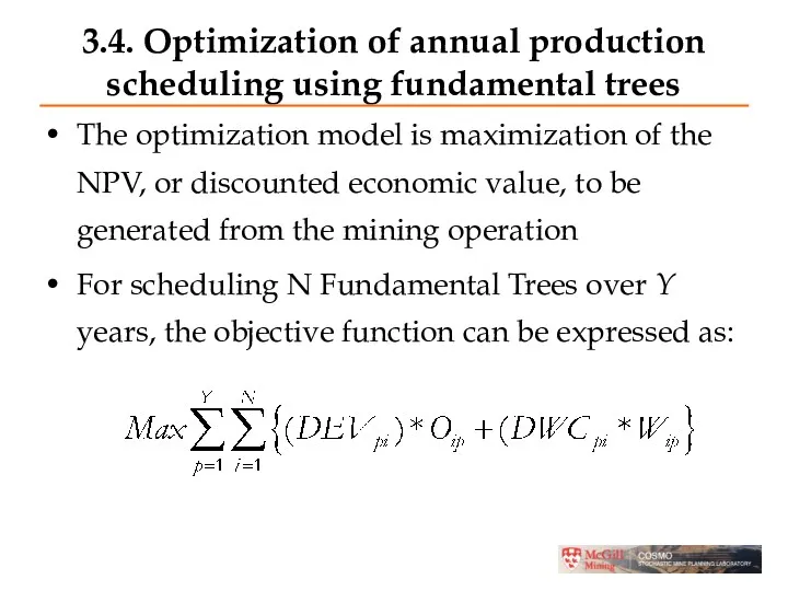
- 47. 3.4. Optimization of annual production scheduling using fundamental trees The optimization model is maximization of the
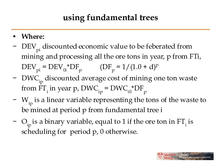
- 48. using fundamental trees Where: DEVpi discounted economic value to be feberated from mining and processing all
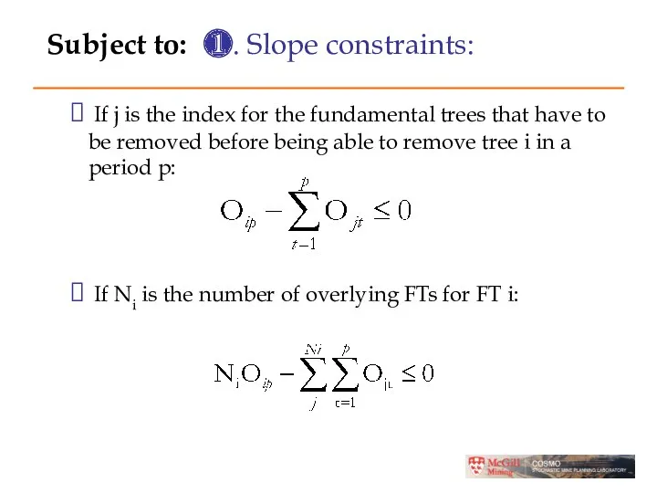
- 49. Subject to: ❶. Slope constraints: If j is the index for the fundamental trees that have
- 50. ❷. Sequencing of mining ore and waste If mining the ore tonnages from a given FT,
- 51. ❸. Grade blending constraints Upper bound constraints: The average grade of the material sent to the
- 52. ❹. Processing capacity constraints Upper bound: The total tonnage of ore processed cannot be more than
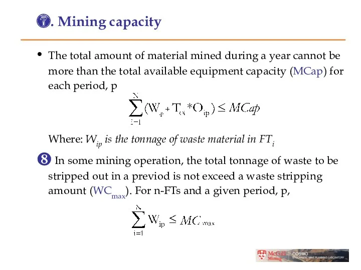
- 53. ❻. The limit on the stripping ratio in each period Where SRmax is the maximum stripping
- 54. ❼. Mining capacity The total amount of material mined during a year cannot be more than
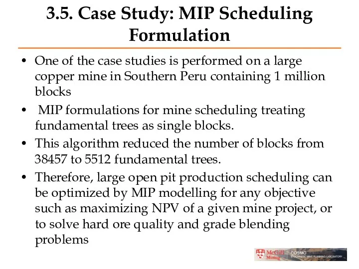
- 55. 3.5. Case Study: MIP Scheduling Formulation One of the case studies is performed on a large
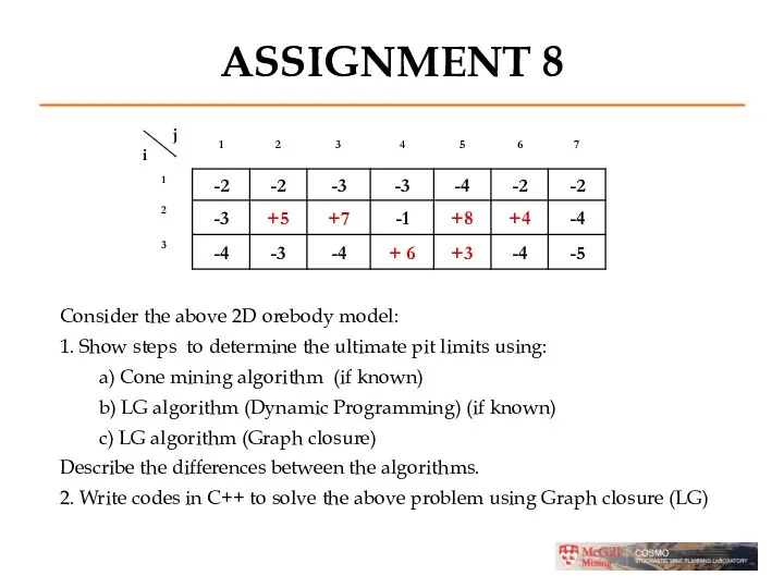
- 56. ASSIGNMENT 8 Consider the above 2D orebody model: 1. Show steps to determine the ultimate pit
- 58. Скачать презентацию
Contents
1. Introduction
2. Lerchs – Grossmann (Graph closure)
3. Fundamental Tree Algorithm
4.
Contents
1. Introduction
2. Lerchs – Grossmann (Graph closure)
3. Fundamental Tree Algorithm
4.
Introduction
Two ojectives for open pit optimization
Design ultimate pit limits (Moving cone,
Introduction
Two ojectives for open pit optimization
Design ultimate pit limits (Moving cone,
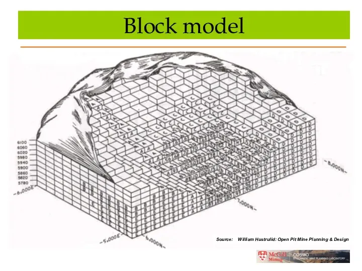
Block model
gdg
Source: William Hustrulid: Open Pit Mine Planning & Design
Block model
gdg
Source: William Hustrulid: Open Pit Mine Planning & Design
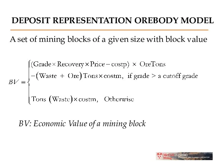
DEPOSIT REPRESENTATION OREBODY MODEL
A set of mining blocks of a given
DEPOSIT REPRESENTATION OREBODY MODEL
A set of mining blocks of a given
DEPOSIT REPRESENTATION OREBODY MODEL
Geologic Model, Copper Grades (lb/ton)
Economic Model, Value per
DEPOSIT REPRESENTATION OREBODY MODEL
Geologic Model, Copper Grades (lb/ton)
Economic Model, Value per
Ultimate Pit Limit Problems
Moving (Floating) Cone Algorithm
Dynamic Programming (LG)
Graph
Ultimate Pit Limit Problems
Moving (Floating) Cone Algorithm
Dynamic Programming (LG)
Graph
2. Graph closure (LG)
The optimal pit outline is the 3D pit
2. Graph closure (LG)
The optimal pit outline is the 3D pit
Lerchs-Grossman Algorithm
Mathematical search technique which works from just two sources of
Lerchs-Grossman Algorithm
Mathematical search technique which works from just two sources of
Arc Relationships
Each arc goes from one block (A) to a
Arc Relationships
Each arc goes from one block (A) to a
Lerchs-Grossman Algorithm
In 3-D each of the blocks is connected to
Lerchs-Grossman Algorithm
In 3-D each of the blocks is connected to
DEFINITIONS
Directed graph G(X, A) is defined by a set of nodes
DEFINITIONS
Directed graph G(X, A) is defined by a set of nodes
BASIC TERMINOLOGY
Vertex, xi is the value of block i.
Arc,
BASIC TERMINOLOGY
Vertex, xi is the value of block i.
Arc,
Root is the vertex without predecessor
A closure is any
Root is the vertex without predecessor
A closure is any
An m-arc is weak if it is supported by positive
An m-arc is weak if it is supported by positive
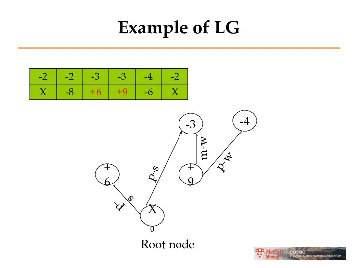
Example of LG
-3
-4
+6
+9
X0
p-s
m-w
p-w
p-s
Root node
Example of LG
-3
-4
+6
+9
X0
p-s
m-w
p-w
p-s
Root node
Steps of the algorithm (1)
-2
-2
-3
-4
+6
+9
X0
Step 0: Connect all nodes to the
Steps of the algorithm (1)
-2
-2
-3
-4
+6
+9
X0
Step 0: Connect all nodes to the
Steps of the algorithm (2)
-2
-3
-3
-4
+6
+9
X0
Step 1: Connect p-strong arcs to all
Steps of the algorithm (2)
-2
-3
-3
-4
+6
+9
X0
Step 1: Connect p-strong arcs to all
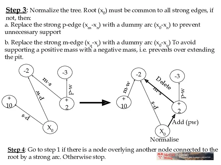
Step 3: Normalize the tree. Root (x0) must be common to
Step 3: Normalize the tree. Root (x0) must be common to
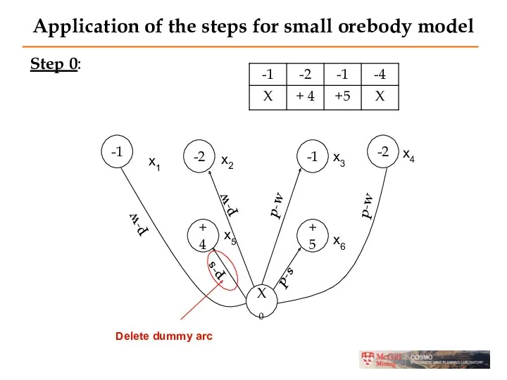
Application of the steps for small orebody model
Step 0:
Application of the steps for small orebody model
Step 0:
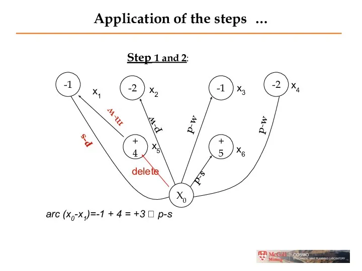
Application of the steps …
Step 1 and 2:
Application of the steps …
Step 1 and 2:
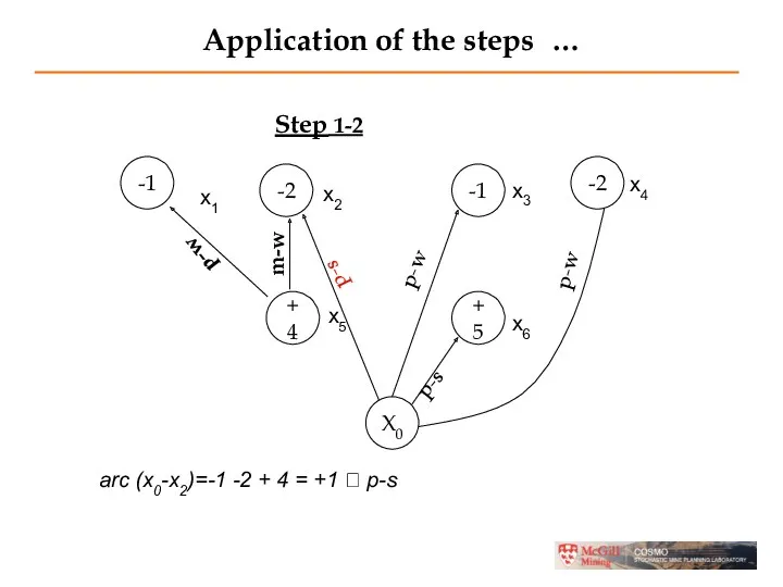
Application of the steps …
Step 1-2
-1
-2
-1
-2
+4
+5
X0
p-w
p-w
p-s
p-s
x2
x1
x3
x4
x5
x6
p-w
arc (x0-x2)=-1 -2 + 4 =
Application of the steps …
Step 1-2
-1
-2
-1
-2
+4
+5
X0
p-w
p-w
p-s
p-s
x2
x1
x3
x4
x5
x6
p-w
arc (x0-x2)=-1 -2 + 4 =
Application of the steps …
Step 1-2
-1
-2
-1
-2
+4
+5
X0
mw
p-w
p-s
x2
x1
x3
x4
x5
x6
p-w
arc (x2-x5)= 4 -1-2 = +1
Application of the steps …
Step 1-2
-1
-2
-1
-2
+4
+5
X0
mw
p-w
p-s
x2
x1
x3
x4
x5
x6
p-w
arc (x2-x5)= 4 -1-2 = +1
Application of the steps …
Step 1-2
arc (x0-x2)= 4 -1-2 + 5
Application of the steps …
Step 1-2
arc (x0-x2)= 4 -1-2 + 5
Application of the steps …
Step 1-2
-1
-2
-1
-2
+4
+5
X0
mw
p-w
p-s
x2
x1
x3
x4
x5
x6
p-w
arc (x0-x2)= 4 -1-2 + 5
Application of the steps …
Step 1-2
-1
-2
-1
-2
+4
+5
X0
mw
p-w
p-s
x2
x1
x3
x4
x5
x6
p-w
arc (x0-x2)= 4 -1-2 + 5
Final Pit Limit
Mine all the nodes connected to a strong arc.
Final Pit Limit
Mine all the nodes connected to a strong arc.
Optimal Pit
The L-G algorithm will flag each block as being
Optimal Pit
The L-G algorithm will flag each block as being
Varying Slope Angles
It is possible to have different slope angles
Varying Slope Angles
It is possible to have different slope angles
3. Fundamental Tree Algorithm
Long-term production scheduling consists of determining an optimal
3. Fundamental Tree Algorithm
Long-term production scheduling consists of determining an optimal
The Approach
To simplify the MIP we would like to decrease the
The Approach
To simplify the MIP we would like to decrease the
The Approach
A Fundamental Tree is defined as a combination of blocks
The Approach
A Fundamental Tree is defined as a combination of blocks
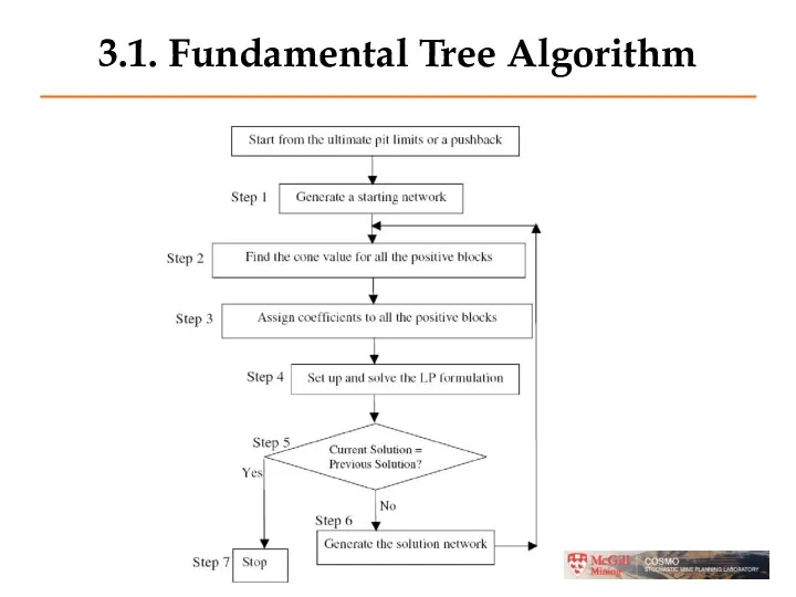
3.1. Fundamental Tree Algorithm
3.1. Fundamental Tree Algorithm
Step 1 - Generate a Starting Network
Given a our pushback block
Step 1 - Generate a Starting Network
Given a our pushback block
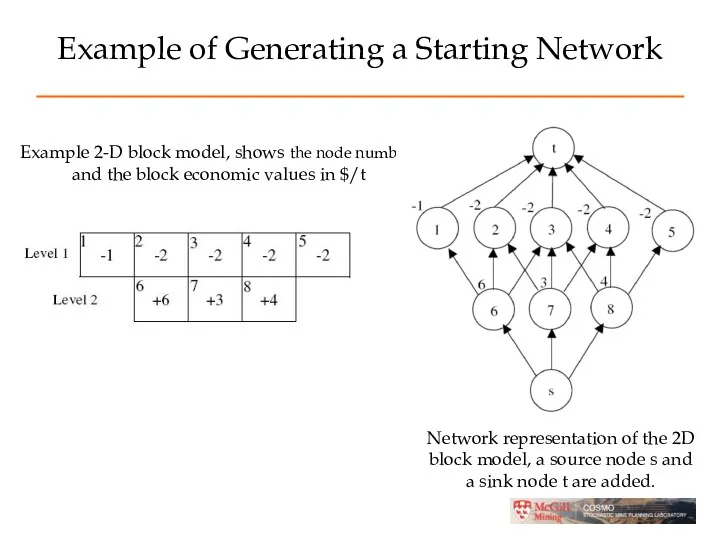
Example of Generating a Starting Network
Example 2-D block model, shows the
Example of Generating a Starting Network
Example 2-D block model, shows the
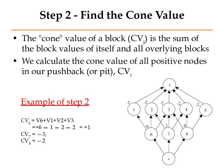
Step 2 - Find the Cone Value
The "cone" value of a
Step 2 - Find the Cone Value
The "cone" value of a
Step 3 – Assign cofficients to the Positive Nodes
Each positive node
Step 3 – Assign cofficients to the Positive Nodes
Each positive node
Example
CV6 = +1; CV7 = —3; CV8 = —2
Coefficients Ci
Example
CV6 = +1; CV7 = —3; CV8 = —2
Coefficients Ci
Step 4 - Set up the LP
Set up a Linear Program
Step 4 - Set up the LP
Set up a Linear Program
Step 5 - Check if we are done
If the number of
Step 5 - Check if we are done
If the number of
3.2. Formulating the Linear Program
* The objective function:
Ci is
3.2. Formulating the Linear Program
* The objective function:
Ci is
Example of Step 4
Example of Step 4
Example of Step 4
The network representation of the initial solution containing
Example of Step 4
The network representation of the initial solution containing
Example of Step 4
The network representation the solution containing three trees
Example of Step 4
The network representation the solution containing three trees
3.3. Properties of the fundamental trees
Property 1 - All fundamental
3.3. Properties of the fundamental trees
Property 1 - All fundamental
Property 2 of the fundamental trees
All fundamental trees obey the
Property 2 of the fundamental trees
All fundamental trees obey the
Property 3 of the fundamental trees
A tree found by FTcannot
Property 3 of the fundamental trees
A tree found by FTcannot
3.4. Optimization of annual production scheduling using fundamental trees
The optimization
3.4. Optimization of annual production scheduling using fundamental trees
The optimization
using fundamental trees
Where:
DEVpi discounted economic value to be feberated from
using fundamental trees
Where:
DEVpi discounted economic value to be feberated from
Subject to: ❶. Slope constraints:
If j is the
Subject to: ❶. Slope constraints:
If j is the
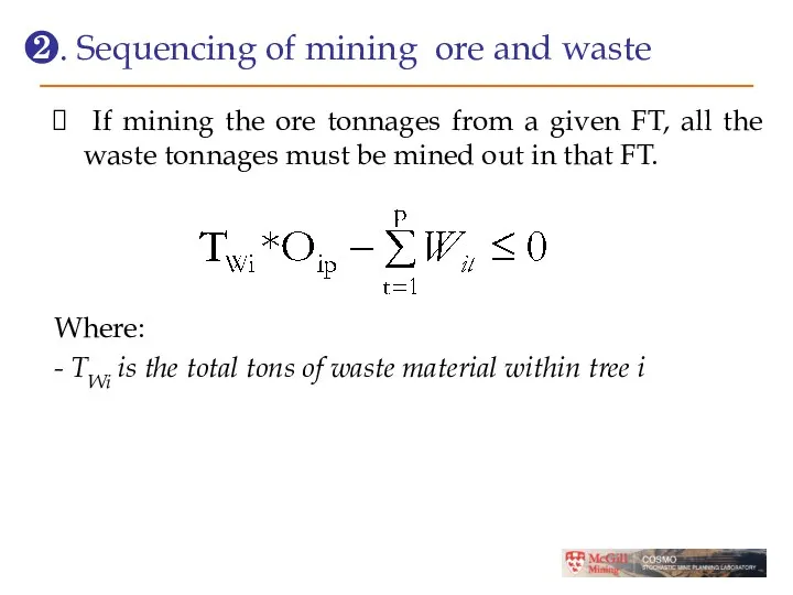
❷. Sequencing of mining ore and waste
If mining the
❷. Sequencing of mining ore and waste
If mining the
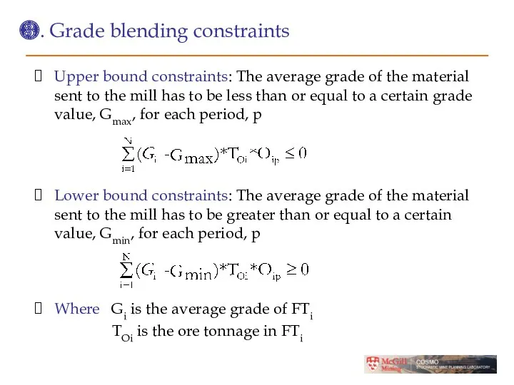
❸. Grade blending constraints
Upper bound constraints: The average grade of
❸. Grade blending constraints
Upper bound constraints: The average grade of
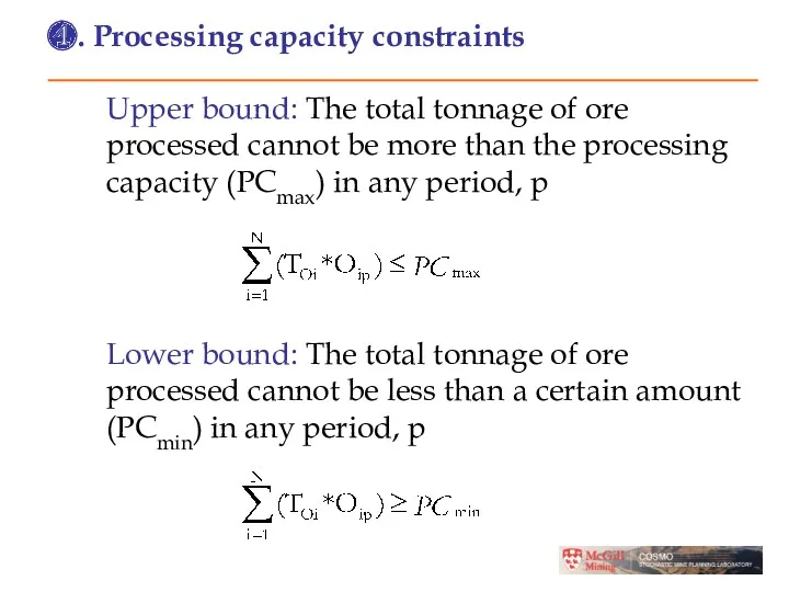
❹. Processing capacity constraints
Upper bound: The total tonnage of ore
❹. Processing capacity constraints
Upper bound: The total tonnage of ore
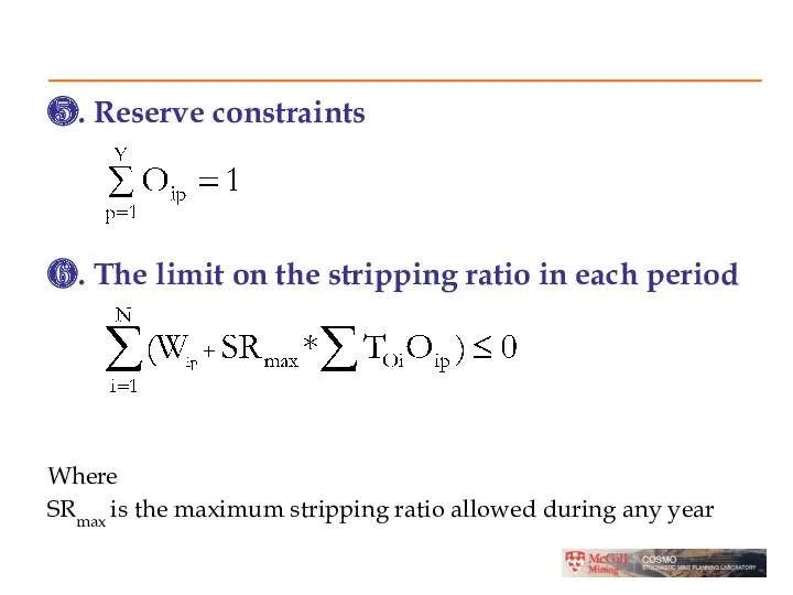
❻. The limit on the stripping ratio in each period
Where
SRmax
❻. The limit on the stripping ratio in each period
Where
SRmax
❼. Mining capacity
The total amount of material mined during a year
❼. Mining capacity
The total amount of material mined during a year
3.5. Case Study: MIP Scheduling Formulation
One of the case studies is
3.5. Case Study: MIP Scheduling Formulation
One of the case studies is
ASSIGNMENT 8
Consider the above 2D orebody model:
1. Show steps to
ASSIGNMENT 8
Consider the above 2D orebody model:
1. Show steps to
 Разработка логической игры Пазлы на платформе UNITY
 Introduction to computer systems. Architecture of computer systems. Lecture2
 Брейн ринг по информатике
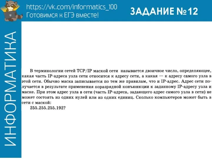 Готовимся к ЕГЭ. Задание №12. IP-адрес
 Презентация по информатике Умники и умницы
 Модели надежности
 Электронный учебник по информатике
 Виды современных компьютеров (от мощных компьютерных систем, до мини-компьютеров)
 Информатика и история развития информационных технологий
 Логические значения. Ветвление (Delphi)
 Модели информационных процессов
 WEB-дизайн. Эргономика WEB-сайта
 HTML: Базові, основні та складні елементи. Лекция 25
 Интернет-технологии. Интернет-маркетинг
 Интеллектуальные методы в экономике и бизнесе
 Навигатор дополнительного образования
 Web index report. Аудитория интернет-проектов. Результаты исследования: Март 2016
 Компьютерные атаки
 История связи. Простейшие средства связи
 Информационные технологии
 Алгоритм и его формальное исполнение
 Спам. Возникновение, распространение, способы защиты
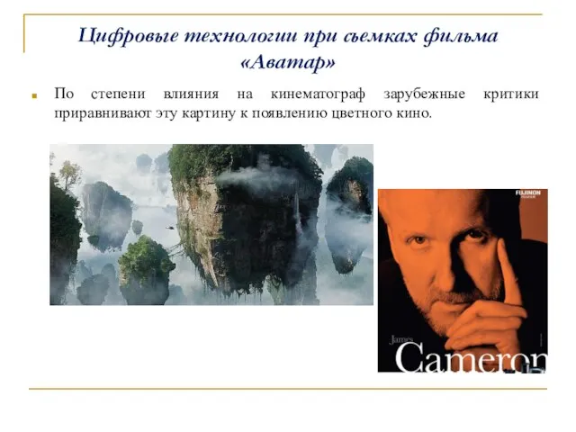 Цифровые технологии при съемках фильма Аватар
 Урок Группы клавиш. Основная позиция пальцев на клавиатуре 5 класс
 Создание мобильной версии сайта
 Объекты и их имена. Признаки объектов. (Урок 1)
 Software upgrade guide
 Внесение данных в информационную систему Мониторинг оказания паллиативной медицинской помощи взрослому населению и детям