- Statistics toolbox

Содержание
- 2. Decision Tree functions
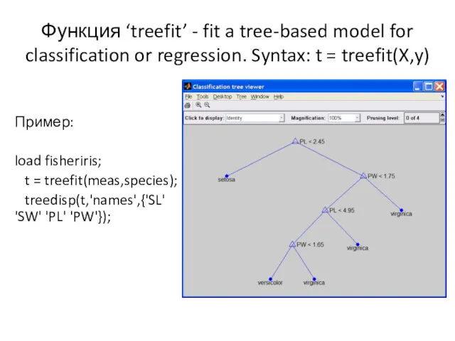
- 3. Функция ‘treefit’ - fit a tree-based model for classification or regression. Syntax: t = treefit(X,y) Пример:
- 4. Cluster analysis functions
- 5. Функция kmeans IDX = kmeans(X,k) [IDX,C] = kmeans(X,k) [IDX,C,sumd] = kmeans(X,k) [IDX,C,sumd,D] = kmeans(X,k) [...] =
- 6. Параметр ‘distance’ 'sqEuclidean‘ - Squared Euclidean distance (default). 'cityblock‘ - Sum of absolute differences, i.e., L1.
- 7. Параметр ‘start’ Method used to choose the initial cluster centroid positions, sometimes known as "seeds". Valid
- 8. Classification load fisheriris; gscatter(meas(:,1), meas(:,2), species,'rgb','osd'); xlabel('Sepal length'); ylabel('Sepal width');
- 9. Linear and quadratic discriminant analysis linclass = classify(meas(:,1:2), meas(:,1:2),species); bad = ~strcmp(linclass,species); numobs = size(meas,1); pbad
- 10. Visualization regioning the plane [x,y] = meshgrid(4:.1:8,2:.1:4.5); x = x(:); y = y(:); j = classify([x
- 11. Decision trees tree = treefit(meas(:,1:2), species); [dtnum,dtnode,dtclass] = treeval(tree, meas(:,1:2)); bad = ~strcmp(dtclass,species); sum(bad) / numobs
- 12. Iris classification tree
- 13. Тестирование качества классификации resubcost = treetest(tree,'resub'); [cost,secost,ntermnodes,bestlevel] = treetest(tree,'cross',meas(:,1:2),species); plot(ntermnodes,cost,'b-', ntermnodes,resubcost,'r--') figure(gcf); xlabel('Number of terminal nodes');
- 14. Выбор уровня [mincost,minloc] = min(cost); cutoff = mincost + secost(minloc); hold on plot([0 20], [cutoff cutoff],
- 15. Оптимальное дерево классификации prunedtree = treeprune(tree,bestlevel); treedisp(prunedtree) cost(bestlevel+1) >> ans = 0.22
- 17. Скачать презентацию
Decision Tree functions
Decision Tree functions
Функция ‘treefit’ - fit a tree-based model for classification or regression.
Функция ‘treefit’ - fit a tree-based model for classification or regression.
Cluster analysis functions
Cluster analysis functions
![Функция kmeans IDX = kmeans(X,k) [IDX,C] = kmeans(X,k) [IDX,C,sumd] =](/_ipx/f_webp&q_80&fit_contain&s_1440x1080/imagesDir/jpg/150355/slide-4.jpg)
Функция kmeans
IDX = kmeans(X,k)
[IDX,C] = kmeans(X,k)
[IDX,C,sumd] = kmeans(X,k)
[IDX,C,sumd,D] = kmeans(X,k)
[...] =
Функция kmeans
IDX = kmeans(X,k)
[IDX,C] = kmeans(X,k)
[IDX,C,sumd] = kmeans(X,k)
[IDX,C,sumd,D] = kmeans(X,k)
[...] =
Параметр ‘distance’
'sqEuclidean‘ - Squared Euclidean distance (default).
'cityblock‘ - Sum of
Параметр ‘distance’
'sqEuclidean‘ - Squared Euclidean distance (default).
'cityblock‘ - Sum of
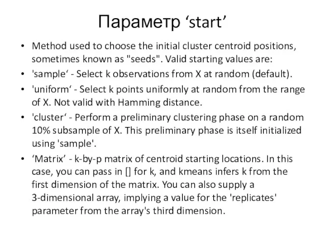
Параметр ‘start’
Method used to choose the initial cluster centroid positions, sometimes
Параметр ‘start’
Method used to choose the initial cluster centroid positions, sometimes
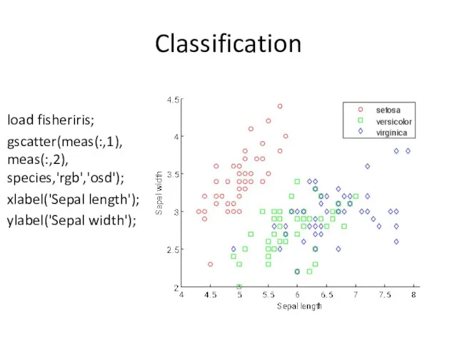
Classification
load fisheriris;
gscatter(meas(:,1), meas(:,2), species,'rgb','osd');
xlabel('Sepal length');
ylabel('Sepal width');
Classification
load fisheriris;
gscatter(meas(:,1), meas(:,2), species,'rgb','osd');
xlabel('Sepal length');
ylabel('Sepal width');
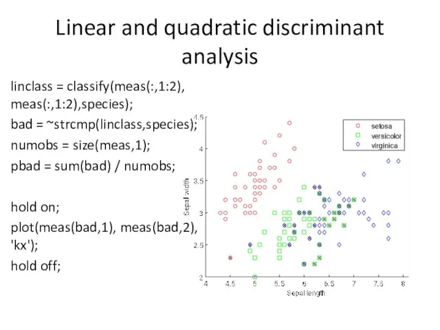
Linear and quadratic discriminant analysis
linclass = classify(meas(:,1:2), meas(:,1:2),species);
bad = ~strcmp(linclass,species);
numobs =
Linear and quadratic discriminant analysis
linclass = classify(meas(:,1:2), meas(:,1:2),species);
bad = ~strcmp(linclass,species);
numobs =
![Visualization regioning the plane [x,y] = meshgrid(4:.1:8,2:.1:4.5); x = x(:);](/_ipx/f_webp&q_80&fit_contain&s_1440x1080/imagesDir/jpg/150355/slide-9.jpg)
Visualization regioning the plane
[x,y] = meshgrid(4:.1:8,2:.1:4.5);
x = x(:);
y = y(:);
j =
Visualization regioning the plane
[x,y] = meshgrid(4:.1:8,2:.1:4.5);
x = x(:);
y = y(:);
j =
![Decision trees tree = treefit(meas(:,1:2), species); [dtnum,dtnode,dtclass] = treeval(tree, meas(:,1:2)); bad = ~strcmp(dtclass,species); sum(bad) / numobs](/_ipx/f_webp&q_80&fit_contain&s_1440x1080/imagesDir/jpg/150355/slide-10.jpg)
Decision trees
tree = treefit(meas(:,1:2), species);
[dtnum,dtnode,dtclass] = treeval(tree, meas(:,1:2));
bad = ~strcmp(dtclass,species);
sum(bad) /
Decision trees
tree = treefit(meas(:,1:2), species);
[dtnum,dtnode,dtclass] = treeval(tree, meas(:,1:2));
bad = ~strcmp(dtclass,species);
sum(bad) /
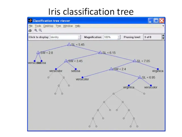
Iris classification tree
Iris classification tree
![Тестирование качества классификации resubcost = treetest(tree,'resub'); [cost,secost,ntermnodes,bestlevel] = treetest(tree,'cross',meas(:,1:2),species); plot(ntermnodes,cost,'b-',](/_ipx/f_webp&q_80&fit_contain&s_1440x1080/imagesDir/jpg/150355/slide-12.jpg)
Тестирование качества классификации
resubcost = treetest(tree,'resub');
[cost,secost,ntermnodes,bestlevel] = treetest(tree,'cross',meas(:,1:2),species);
plot(ntermnodes,cost,'b-', ntermnodes,resubcost,'r--')
figure(gcf);
xlabel('Number of terminal nodes');
ylabel('Cost
Тестирование качества классификации
resubcost = treetest(tree,'resub');
[cost,secost,ntermnodes,bestlevel] = treetest(tree,'cross',meas(:,1:2),species);
plot(ntermnodes,cost,'b-', ntermnodes,resubcost,'r--')
figure(gcf);
xlabel('Number of terminal nodes');
ylabel('Cost
![Выбор уровня [mincost,minloc] = min(cost); cutoff = mincost + secost(minloc);](/_ipx/f_webp&q_80&fit_contain&s_1440x1080/imagesDir/jpg/150355/slide-13.jpg)
Выбор уровня
[mincost,minloc] = min(cost);
cutoff = mincost + secost(minloc);
hold on
plot([0 20],
Выбор уровня
[mincost,minloc] = min(cost);
cutoff = mincost + secost(minloc);
hold on
plot([0 20],
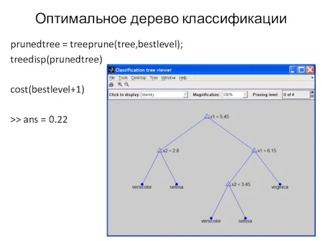
Оптимальное дерево классификации
prunedtree = treeprune(tree,bestlevel);
treedisp(prunedtree)
cost(bestlevel+1)
>> ans = 0.22
Оптимальное дерево классификации
prunedtree = treeprune(tree,bestlevel);
treedisp(prunedtree)
cost(bestlevel+1)
>> ans = 0.22
 Создание и обработка изображений средствами Adobe Photoshop (обзор возможностей)
 Хімічна інформатика
 Analysis and Design of Data Systems. Enhanced ER (EER) Mode. (Lecture 11)
 История создания UNIX-систем. (Занятия 3 и 4)
 Реферативная база данных
 Операционные системы. Управление процессами
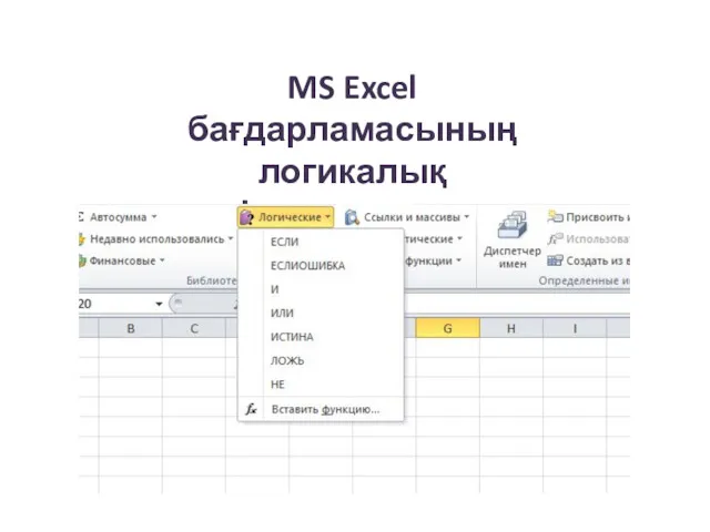 MS Excel бағдарламасының логикалық функциялары
 Электронное портфолио студентов
 Количество информации
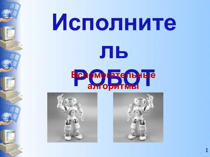 Исполнитель Робот. Вспомогательные алгоритмы
 Встроенный язык 1С. Особенности. Основные приемы работы. Основные конструкции встроенного языка. Лекция 2.1
 Принципы автоматизированного управления приточно-вытяжной вентиляцией
 Понятие и свойства алгоритма
 Обучение SCRATCH
 Форматирование документа
 Фрагментация и персонификация контента в интернете
 Компьютеризация животноводства в РФ
 Алгоритмы и программирование, язык Паскаль (часть 3)
 Основные понятия культура и информация
 Устройства ввода-вывода
 Программное обеспечение компьютера
 Тестирование и тестировщики. Категории программных ошибок
 Сетевая этика. Культура общения в сети
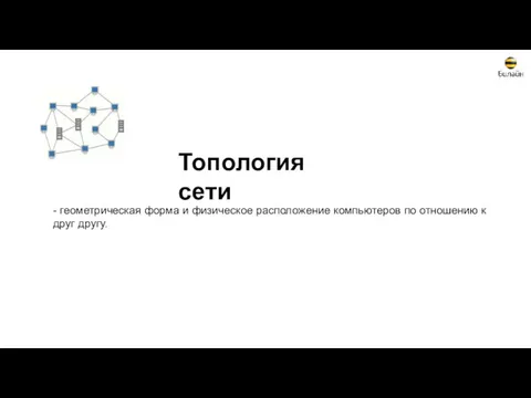 Топология сети. Блок 2
 Введение в дисциплину Информатика и ИКТ
 Правила составления библиографического списка литературы и оформления библиографических ссылок
 Розроблення атоматизованої системи керування робочим процесом в закладах громадського харчування
 Алгоритмы. Алгоритм ветвления.